

Translate this page into:
Multimodal pathomics feature integration for enhanced predictive performance in gastric cancer pathology through radiomic and CNN-derived features
*Corresponding author: E-mail address: m153456895@126.com (L. Peng)
-
Received: ,
Accepted: ,
Abstract
This study aims to improve the accuracy and reliability of gastric cancer grading by creating a computational framework that combines radiomic features and deep learning data from pathology images. By merging traditional and modern modeling techniques, we seek to overcome current diagnostic challenges and build a model that can be used effectively in clinical settings. The dataset included 798 whole-slide images (WSIs) of gastric cancer, divided into over 278,000 smaller image patches categorized into four grades. Radiomic features were collected using the HistomicsTK tool to ensure standard and consistent data collection. At the same time, deep learning features were extracted from fine-tuned CNN models (Xception, InceptionV3, DenseNet169, and EfficientNet) designed for image classification. Advanced methods like LASSO, ANOVA, mutual information (MI), and recursive feature elimination (RFE) were used to pick the most useful features. Different machine learning models, such as XGBoost, LightGBM, CatBoost, Random Forest, Support Vector Machine (SVM), and multi-layer perceptron (MLP), were trained and tested using a five-fold cross-validation process. Performance was assessed using metrics like AUC, accuracy (ACC), and F1-score, with hyperparameters fine-tuned through grid search for the best results. In the analysis using only radiomic features, XGBoost and CatBoost showed the best results, especially with RFE feature selection, achieving test AUCs of 91.1% and 91.2%, respectively, with F1-scores above 90%. When radiomic features were combined with deep learning features from all CNN models, the performance improved significantly. CatBoost with ANOVA reached a training AUC of 97.73% and a test AUC of 95.26%, while XGBoost with RFE achieved a test AUC of 96.9%. The top selected features, which included morphometric, gradient, intensity-based, and Haralick descriptors, were confirmed for their importance through q-value analysis. The combined model showed excellent general performance, with a test AUC of 94.22%, ACC of 95.80%, and an F1-score of 93.10%, proving the strength of using combined multimodal features. This study shows the advantages of combining radiomic and deep learning features for better grading of gastric cancer. In the future, this framework could be expanded to other types of cancer and integrated into clinical workflows, potentially reducing diagnostic errors and improving patient outcomes.
Keywords
Computational pathology
Deep learning
Gastric cancer
Machine learning
Pathology imaging
Radiomics

1. Introduction
Gastric cancer is a major cause of cancer-related deaths globally, especially in East Asia, where incidence and mortality rates are high. Accurate early detection and precise grading of gastric cancer are essential for effective treatment planning and improving patient survival. Traditionally, the diagnosis and grading of gastric cancer have relied on visual assessments by experienced pathologists. However, this manual process is subjective, which can lead to variations in diagnosis between different experts and reduce reliability [1,2]. This has led to growing interest in using computational techniques—specifically machine learning (ML) and deep learning (DL)—to make cancer grading more precise, consistent, and efficient [3-6].
Radiomics is a cutting-edge technique that extracts a wide range of measurable features from medical images to capture detailed patterns in pathology. These features, which describe texture, shape, and intensity, can reveal biological details that are not visible to the human eye. By connecting imaging data with clinical outcomes, radiomics provides data-driven insights into cancer grading and prognosis [7-16].
Deep learning, particularly with convolutional neural networks (CNNs), has greatly improved the field of medical imaging by allowing automated extraction of feature hierarchies, from simple textures to complex patterns [17,18]. This provides deep, detailed information useful for distinguishing between different cancer grades. CNN models like Xception, InceptionV3, DenseNet169, and EfficientNet are known for their ability to capture both large-scale structures and intricate local details, making them well-suited for complex classification tasks. These deep features enhance the analysis of pathology images, helping to differentiate between normal tissue and various tumor grades [19,20].
Although radiomics and deep learning features are powerful when used alone [17,18,21], combining them into a unified framework for grading gastric cancer has not been thoroughly studied. Most past research has focused on either radiomics or deep learning features without examining how their integration might boost diagnostic accuracy [22,23]. Additionally, while some CNN models have been used for end-to-end classification, few studies have explored their use alongside traditional ML classifiers or in ensemble approaches. Integrating these methods could capture a wider range of image characteristics and improve diagnostic precision in cancer grading. Traditional pathology often suffers from subjectivity and inter-observer variability, where pathologists’ interpretations of histopathological images can differ. By combining radiomic features, which provide quantitative and reproducible measures, with deep learning models [21,24-27], which can automatically learn complex patterns and subtle features from large datasets, our approach reduces subjectivity. This integration leads to more objective, consistent, and accurate analyses, ultimately supporting pathologists in making more reliable diagnostic decisions.
Several recent studies have explored the integration of radiomic and deep learning features for cancer grading, particularly in the context of pathomics. For instance, Tan et al. [28] developed AI-based pathomics models combining hematoxylin-eosin (HE) and Ki67 image features with clinical variables for predicting the pathological staging of colorectal cancer. Their combined model demonstrated superior performance, achieving an AUC of 0.907 in the training cohort, and showed high clinical utility in decision-making. Similarly, Chen et al. [29] proposed Pathomic Fusion, a novel approach for fusing histology and genomic features, utilizing deep learning to predict cancer prognosis. By integrating whole-slide images (WSIs) with genomic data such as mutations, copy number variations (CNVs), and RNA-Seq, they demonstrated that multimodal data fusion improved survival outcome prediction in glioma and renal cell carcinoma datasets. Additionally, Zhang et al. [30] focused on gastric cancer, developing a model that integrated histopathological features with transcriptomic data. Their approach, using multi-instance learning and a Lasso-Cox regression model, achieved promising results in prognostic stratification, identifying SLITRK4 as a potential biomarker for gastric cancer. These studies underscore the growing importance of combining multimodal data, such as radiomics and genomic features, for improving cancer grading and prognosis.
This study presents an innovative framework that combines ML, DL, and radiomics to improve the accuracy of gastric cancer grading in pathology images. To our knowledge, this is the first comprehensive approach of its kind for gastric cancer grading. The main contributions include:
Comprehensive feature configurations: We evaluate different feature configurations: (i) radiomic features alone, (ii) DL features from individual CNN models, and (iii) a combined approach that integrates radiomic and DL features from multiple CNN models (Xception, InceptionV3, DenseNet169, EfficientNet). This analysis helps us understand the individual and combined effects of these features in cancer grading.
Direct and ensemble DL models: We test the direct application of CNN models for end-to-end grading and assess an ensemble approach that combines multiple CNNs. This ensemble approach takes advantage of the strengths of each model, improving the robustness and accuracy of cancer grading.
Advanced feature selection and optimization: To manage the high number of radiomic and DL features, we use advanced feature selection methods like LASSO, ANOVA, mutual information (MI), and recursive feature elimination (RFE) to reduce feature redundancy and enhance model performance.
Enhanced model interpretability: We incorporate attention mechanisms in CNN models to focus on the most important regions in pathology images, ensuring that the model’s decisions align with clinically relevant areas. We also use interpretability tools like SHapley Additive exPlanations (SHAP) values to show feature importance, making the models more transparent and clinically useful.
Rigorous validation with key metrics: We validate model performance using five-fold cross-validation and evaluate it with metrics such as accuracy, AUC, and F1-score. Hyperparameter tuning is done with grid search to optimize model configurations, ensuring reliable and generalizable results.
By combining radiomics, DL, and ensemble modeling into one framework, this study sets a new standard for computational pathology in gastric cancer. The proposed approach serves as a robust and scalable tool to support pathologists, offering a data-driven foundation for more accurate diagnoses and evidence-based cancer management. This research not only advances gastric cancer pathology but also paves the way for future studies that integrate multimodal imaging features for better cancer diagnostics.
2. Materials and Methods
2.1. Dataset preparation and preprocessing
The dataset for this study consisted of 798 WSIs stained with HE and scanned at a magnification of 20x. The data used in this study were obtained from a multi-center source, ensuring diversity and enhancing the generalizability of the model. This level of magnification provided the detail needed to observe cellular structures crucial for the accurate grading of gastric cancer. Each WSI was divided into smaller image patches and classified into four categories: normal, grade II, grade III, and grade IV. The study established specific criteria for including and excluding data to ensure consistency and reliability in the analysis. Only WSIs of good quality, showing clear cellular structures and standard HE staining, were included. These images needed to come from patients with confirmed gastric cancer diagnoses, covering different histological grades (e.g., normal tissue, grades II, III, and IV) to allow for a comprehensive classification. Clinical data such as age, gender, and tumor grading were also necessary to strengthen the analysis. Preference was given to images collected within a set timeframe to maintain consistency in sample collection. Only cases with ethical approval and informed patient consent were eligible.
On the other hand, WSIs that were of poor quality, had significant artifacts, or low resolution were excluded because they could interfere with feature extraction and accurate analysis. Pathology images stained using non-standard or inconsistent methods were also not considered. Cases missing essential clinical information, involving metastatic or recurrent gastric cancer, or with unclear histopathological diagnoses were excluded to keep the focus on primary tumor analysis. Additionally, any images that were not from histopathological sources or were from patients who had undergone prior treatment (e.g., chemotherapy or radiation) were excluded, as these could change tissue structures and introduce bias.
The final dataset included a total of 278,126 image patches distributed as follows:
-
-
Normal: 72,126 patches
-
-
Grade II: 71,146 patches
-
-
Grade III: 68,258 patches
-
-
Grade IV: 66,596 patches
Each category had patches of two sizes- 180 × 180 pixels and 140 × 140 pixels—split evenly:
-
-
Normal: 36,063 patches of each size
-
-
Grade II: 35,573 patches of each size
-
-
Grade III: 34,129 patches of each size
-
-
Grade IV: 33,298 patches of each size
The dataset was divided into training, validation, and test sets in a 4:4:2 ratio. The distribution was as follows:
Training Set (40%):
-
-
Normal: 28,850 patches (14,425 of each size)
-
-
Grade II: 28,458 patches (14,229 of each size)
-
-
Grade III: 27,303 patches (13,652 of each size)
-
-
Grade IV: 26,638 patches (13,319 of each size)
-
-
Total: 111,249 patches
Validation Set (40%):
-
-
Normal: 28,850 patches (14,425 of each size)
-
-
Grade II: 28,458 patches (14,229 of each size)
-
-
Grade III: 27,303 patches (13,652 of each size)
-
-
Grade IV: 26,638 patches (13,319 of each size)
-
-
Total: 111,249 patches
Test Set (20%):
-
-
Normal: 14,426 patches (7,213 of each size)
-
-
Grade II: 14,230 patches (7,115 of each size)
-
-
Grade III: 13,652 patches (6,826 of each size)
-
-
Grade IV: 13,320 patches (6,660 of each size)
-
-
Total: 55,628 patches
Data augmentation was used on the training set only to increase diversity and improve the model’s learning. This included transformations such as random 90° rotations and horizontal/vertical flipping. These techniques effectively doubled the number of training patches, leading to:
-
-
Normal: 57,700 augmented patches
-
-
Grade II: 56,916 augmented patches
-
-
Grade III: 54,606 augmented patches
-
-
Grade IV: 53,276 augmented patches
The total number of patches in the augmented training set increased to 222,498. This augmentation helped the model learn from a varied dataset, better preparing it to handle real-world variations in pathology images. By maintaining balanced training, validation, and test sets, this preparation ensures a solid foundation for developing a reliable model for classifying gastric cancer across different grades and patch sizes. An illustration of the AI-driven classification framework is shown in Figure 1.
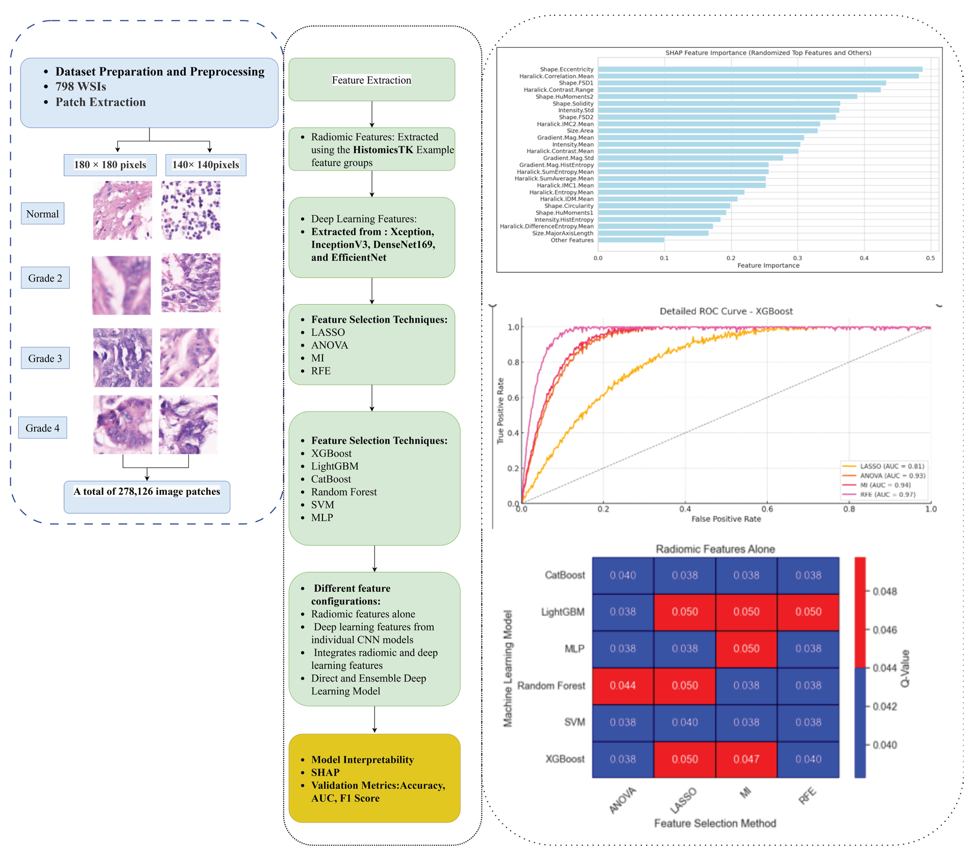
- Step-by-step workflow. WSI: Whole-slide image, LASSO: Least absolute shrinkage and selection operator, ANOVA: Analysis of variance, MI: Mutual information, RFE: Recursive feature elimination, SHAP: SHapley Additive exPlanations, CNN: convolutional neural networks, AUC: Area under the curve.
2.2. Comprehensive feature configurations (radiomic and deep feature extraction)
This study uses a comprehensive approach to develop a strong framework for grading gastric cancer by incorporating both radiomic and DL features. Each part of this methodology contributes to improving the accuracy and interpretability of cancer classification, providing a solid basis for data-driven decisions in pathology.
We tested different input feature configurations to understand the separate and combined effects of radiomic and DL features on gastric cancer classification. The main configurations are outlined below:
Radiomic features: Radiomic feature extraction was used to quantitatively analyze tissue characteristics in pathology images with the HistomicsTK package (Figure 2), an open-source tool available on its GitHub repository. This package adheres to the Image Biomarker Standardization Initiative (IBSI) guidelines to ensure a standardized and repeatable process for feature extraction. Radiomic features are vital for identifying variations at the nuclear and tissue levels, which often signal cancer progression and the degree of differentiation.
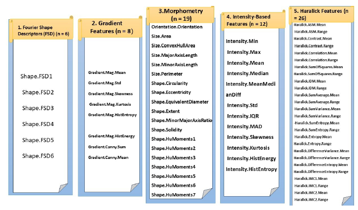
- Selected pathomics features.
By focusing on detailed properties such as shape, texture, and intensity, radiomic analysis helps to boost the predictive accuracy of ML models used for cancer classification. These feature groups provide comprehensive descriptors that measure shape, texture, and intensity differences within pathology images. The extracted features serve as a rich dataset for training ML models, aiding in distinguishing between different cancer grades by examining the fine details of tissue samples.
Deep learning features alone: To effectively classify gastric cancer grades (normal and grades II to IV), we fine-tuned several CNN models, including Xception, InceptionV3, DenseNet169, and EfficientNet. We started with these pre-trained models, excluding their top classification layers, and initialized them with ImageNet weights. To adapt the models for our dataset, we froze all layers except the last 30, allowing these layers to be fine-tuned while preserving the useful, generalized features learned from ImageNet.
We selected Xception, DenseNet169, and EfficientNet based on their demonstrated success in image classification tasks and their suitability for extracting high-level features from pathological images. Xception was chosen for its efficient use of depthwise separable convolutions, while DenseNet169 was selected for its feature reuse architecture, which improves gradient flow and mitigates the vanishing gradient problem. EfficientNet was included for its ability to balance model size and accuracy, offering state-of-the-art performance with fewer parameters.
We added custom layers to the modified base models to better capture patterns specific to gastric cancer. These custom layers included a Global Average Pooling layer to reduce the spatial size of the feature maps, followed by a Dropout layer (rate of 0.5) to prevent overfitting. We also added a Dense layer with 256 neurons and ReLU activation to introduce non-linearity and enhance the learning of complex patterns, followed by another Dropout layer (rate of 0.3) for further regularization. This setup created a modified model called the features_model, designed to extract deep features tailored for gastric cancer classification.
Our dataset, divided into training and test sets with images labeled across four classes, was processed through the features_model to extract deep features up to the final custom layer. These deep features captured high-level information, emphasizing characteristics essential for distinguishing different cancer grades.
By fine-tuning instead of freezing the entire network and simply adding layers, we allowed the models to adjust their internal representations to better match the specific traits of gastric tissue images. This method provided a more refined and accurate performance compared to using the networks as fixed feature extractors. These extracted features were individually tested with ML classifiers to assess their effectiveness in classification, ensuring that each CNN’s capability in recognizing meaningful patterns was thoroughly evaluated for improved cancer grading accuracy.
Integrated radiomic and deep features from all CNN models: In the final step, we combined radiomic features with deep features extracted from all CNN models. This created a comprehensive feature set that included a wide range of imaging information, capturing detailed characteristics from both radiomic and DL perspectives. By integrating these diverse features, we aimed to explore how combining multiple DL architectures with radiomic data could enhance classification performance through a fuller representation of image characteristics.
2.3. Direct and ensemble deep learning models
In addition to using extracted features with ML models, we also evaluated the performance of direct, end-to-end CNN models and ensemble strategies for grading gastric cancer:
Direct CNN models: Each CNN model was fine-tuned and directly applied to classify pathology images into different cancer grades. These models performed classification end-to-end, without relying on additional ML layers. This approach helped us understand the capabilities of each individual CNN architecture in handling the complete task of grading cancer from input to output.
Ensemble strategy: To make the models more robust, we used an ensemble strategy that combined predictions from multiple CNN models. This approach took advantage of the strengths of each architecture while minimizing their individual weaknesses. By combining CNNs with different structures and depths, the ensemble model aimed to improve accuracy and consistency across various cancer grades. We used voting-based or averaging techniques for final predictions, depending on what worked best during our experiments.
2.4. Advanced feature selection and optimization
To manage the high number of features from combined radiomic and DL sources, feature selection techniques were used to reduce redundancy and boost model performance. Least Absolute Shrinkage and Selection Operator (LASSO) was applied as a regularization method. It works by penalizing the size of regression coefficients, effectively setting non-informative or redundant features to zero, thus simplifying the feature set while keeping its predictive strength intact. Analysis of Variance (ANOVA) was used to evaluate the statistical importance of each feature by comparing the variance between different classes. This helped select features with strong discriminative power based on their ANOVA scores. MI measured how dependent a feature was on the target class, ensuring that only features providing unique and valuable information were selected. Features with high MI scores were chosen for their significant contribution to model performance. RFE was an iterative method to refine the feature set by ranking features according to their importance and gradually removing the least useful ones until the most effective subset was found. This step-by-step process helped develop a feature set that maximized accuracy while reducing computational load.
Although RFE showed the best results for feature selection in this study, we acknowledge that it has certain drawbacks compared to simpler methods like LASSO and ANOVA. Specifically, RFE can be computationally intensive, as it involves iterative model training, which may be challenging for large datasets or more complex models. Additionally, while RFE is less prone to overfitting compared to exhaustive feature selection methods, overfitting may still occur if the number of retained features is large relative to the dataset size. To address this, we employed cross-validation during the feature selection process. In contrast, methods like LASSO and ANOVA are computationally simpler but may not capture the complex interactions between features as effectively as RFE.
We trained various ML models to test the effectiveness of these selected features for classifying gastric cancer grades. The models were: (i) XGBoost- Known for its strong ensemble learning abilities and high performance (ii) LightGBM: Optimized for speed and memory efficiency (iii) CatBoost: Effective with categorical data, providing reliable classification results (iv) Random Forest: An ensemble method using multiple decision trees, balancing accuracy and avoiding overfitting (iv) Support Vector Machine (SVM): Capable of handling high-dimensional feature spaces and finding optimal class-separating hyperplanes (v) Multilayer Perceptron (MLP): A type of neural network suited for complex, non-linear classification tasks. These classifiers were tested with the optimized feature sets obtained from the selection process. Combining comprehensive feature extraction, careful selection, and thorough model training and validation provided a robust system for accurately classifying gastric cancer grades. This approach ensured that the final models were efficient, predictive, and suitable for reliable pathology image analysis.
To address potential overfitting due to data augmentation, we employed cross-validation and early-stopping techniques during model training. Regularization methods, such as dropout and L2 regularization, were also applied. Furthermore, we ensured that the augmented images maintained realistic variations consistent with typical pathological data, thereby improving model generalizability without introducing artificial bias.
2.5. Enhanced model interpretability
To ensure that the model’s decision-making process aligns with clinically important information, we used several interpretability techniques: SHAP (SHapley Additive exPlanations): SHAP values were used to understand the contribution of each feature to the model’s predictions. SHAP offers a consistent way to measure feature importance across different models, making it clear which radiomic or DL features are influencing the classification. This tool is particularly important in clinical settings where understanding how the model makes decisions helps build trust and ensures transparency. These interpretability techniques help make sure that the model’s outputs are not only accurate but also meaningful from a clinical standpoint. They provide insights that align with expert knowledge, which supports the practical use of AI in pathology.
2.6. Rigorous validation with key metrics
To measure how well the models performed, we used the following key metrics:
-
-
Accuracy (ACC): The percentage of patches correctly classified into the correct cancer grades.
-
-
Area Under the Curve (AUC): AUC values were calculated from receiver operating characteristic (ROC) curves to evaluate the model’s ability to distinguish between different cancer grades.
-
-
F1 Score: This score, which combines precision and recall, was used to give a balanced view of the model’s effectiveness, especially when handling class imbalances.
Hyperparameter tuning via grid search: To find the best configurations for each model, we used grid search for hyperparameter tuning. This process involved systematically testing different combinations of hyperparameters and selecting the one that provided the highest performance based on validation results. Grid search was applied to all feature configurations and models, ensuring a thorough optimization process. By combining these steps, this study offers a comprehensive approach to grading gastric cancer. It integrates advanced feature configurations, ensemble learning, feature selection, interpretability methods, and thorough validation to develop a reliable and clinically useful model for pathology image classification.
The system used for running the models included high-performance computing resources for efficient processing and accurate results. It featured a multi-core CPU (AMD Ryzen) and multiple NVIDIA GPUs (Tesla V100) to manage the demands of DL and ML tasks. The system also had at least 128 GB of RAM for large-scale data processing and high-speed SSD storage for quick access to pathology image data. Software frameworks such as TensorFlow were used for training DL models, while Scikit-learn and XGBoost supported traditional ML tasks. The models were run on a Linux-based operating system for its stability and performance benefits.
3. Results and Discussion
3.1. Selected features and SHAP analysis
After applying various feature selection methods, a refined set of 25 top features was identified as the most informative inputs for the ML models (Table 1). These features came from multiple categories, providing a comprehensive representation of image characteristics essential for effective classification. The selected features included Fourier Shape Descriptors (FSD), Gradient Features, Morphometry, Intensity-Based Features, and Haralick Features. This curated selection ensures a balanced input that captures both shape and texture information, enhancing the predictive accuracy and overall performance of the models in grading gastric cancer.
| Feature Group | Number of Features | Features |
|---|---|---|
| Fourier Shape Descriptors (FSD) | 2 | Shape.FSD1, Shape.FSD2 |
| Gradient Features | 3 | Gradient.Mag.Mean,Gradient.Mag.Std, Gradient.Mag.HistEntropy |
| Morphometry | 7 | Size.Area, Size.MajorAxisLength, Shape.Circularity, Shape.Eccentricity, Shape.Solidity, Shape.HuMoments1, Shape.HuMoments2 |
| Intensity-Based Features | 3 | Intensity.Mean, Intensity.Std, Intensity.HistEntropy |
| Haralick Features | 10 | Haralick.Contrast.Mean, Haralick.Correlation.Mean, Haralick.SumAverage.Mean, Haralick.Entropy.Mean, Haralick.DifferenceEntropy.Mean, Haralick.SumEntropy.Mean,Haralick.IMC1.Mean, Haralick.IMC2.Mean,Haralick.Contrast.Range, Haralick.IDM.Mean |
The analysis of dependence plots for the top 25 features offers valuable insights into how these features influence the model’s predictions (Figure 3). Each feature has a unique impact, with some, like Shape.FSD1, Gradient.Mag. Mean, and Haralick.Correlation. Mean, showing significant effects on model output. SHAP values reveal the strength of each feature’s contribution, where higher values signal a greater influence on the model’s decisions. The observed patterns indicate both linear and non-linear relationships, suggesting that some features have a simple correlation with the target while others interact in more complex ways. The color variations in the plots point to potential interactions between features, providing a deeper understanding of how certain attributes may work together or counteract each other in shaping predictions. These observations highlight the importance of careful feature selection and analysis in building robust ML models and optimizing their predictive performance.
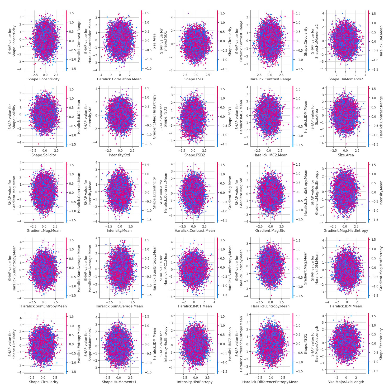
- Dependence plots for top 25 features illustrating SHAP values and feature interactions in model predictions. SHAP: SHapley Additive exPlanations.
Figure 4 illustrates a SHAP feature importance plot, which underscores the contributions of the top 25 features used in our predictive model. This visualization is essential for understanding how the model makes decisions by identifying which features have the greatest influence on its outputs. Prominent features such as ‘Shape.Eccentricity’ and ‘Haralick.Correlation.Mean’ emerge as significant contributors, showing the highest SHAP values. The plot also summarizes the contributions of less impactful features under an “Other Features” category, offering a comprehensive view of feature importance throughout the model. By using SHAP values, this analysis ensures a transparent and interpretable method for evaluating feature influence, aiding in the targeted refinement of feature selection and model improvement.
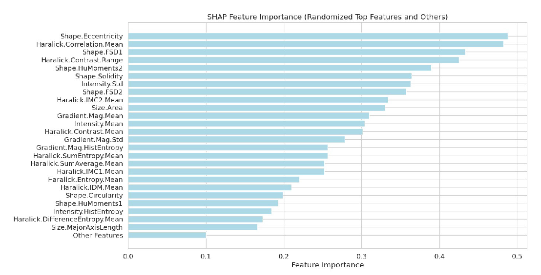
- SHAP-based feature importance analysis for enhanced model interpretability. SHAP: SHapley Additive exPlanations.
3.2. Radiomic features alone
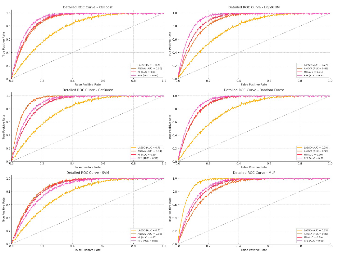
XGBoost and CatBoost were the best-performing models when combined with RFE. Both models showed high AUC, ACC, and F1-score metrics, highlighting their strength in handling complex radiomic features (Table 2). XGBoost with RFE achieved an AUC of 91.9% on the training set, 91.2% on the validation set, and 91.1% on the test set, along with strong ACC and F1-scores of 90.23% and 89.14% on the training set, respectively. Similarly, CatBoost had AUCs of 92%, 91.5%, and 91.2% for training, validation, and test sets, respectively, with an F1-score of 90.5% on the test set (Figure 5).
| Machine learning models | Feature Selection | AUC (%) | ACC (%) | F1score (%) | ||||||
|---|---|---|---|---|---|---|---|---|---|---|
| Training | Validation | Testing | Training | Validation | Testing | Training | Validation | Testing | ||
| XGBoost | LASSO | 78.3 | 77.5 | 75.5 | 77.25 | 76.23 | 75.58 | 76.76 | 75.25 | 74.9 |
| ANOVA | 89.25 | 88.25 | 87.8 | 88.23 | 87.29 | 86.92 | 89.27 | 88.9 | 88.5 | |
| MI | 90.6 | 89.32 | 89.25 | 89.89 | 89.5 | 89.2 | 87.31 | 86.98 | 86.45 | |
| RFE | 91.9 | 91.20 | 91.10 | 90.23 | 89.25 | 89.32 | 89.14 | 88.75 | 88.5 | |
| LightGBM | LASSO | 77.5 | 76.25 | 76.2 | 78.23 | 77.87 | 77.5 | 79.34 | 78.65 | 78 |
| ANOVA | 87.3 | 87.2 | 86.25 | 86.14 | 85.9 | 85.5 | 87.8 | 86.8 | 85.64 | |
| MI | 89.21 | 89 | 88.69 | 88.5 | 88.2 | 87.25 | 89.21 | 89.10 | 88.78 | |
| RFE | 90.5 | 89.74 | 89.5 | 86.25 | 86.15 | 85.69 | 87.24 | 87.12 | 86.52 | |
| CatBoost | LASSO | 76.65 | 76.25 | 75.9 | 77.25 | 76.58 | 76.56 | 78.5 | 77.25 | 76.1 |
| ANOVA | 88.5 | 88.2 | 87.5 | 87.23 | 87.10 | 86.9 | 86.9 | 86.5 | 86.23 | |
| MI | 90.5 | 89.23 | 88.78 | 88.89 | 88.25 | 87.5 | 89.23 | 89.10 | 88.90 | |
| RFE | 92 | 91.5 | 91.2 | 91 | 90.32 | 90.2 | 92 | 91.5 | 90.5 | |
| Random Forest | LASSO | 78.45 | 78.25 | 76.5 | 76.5 | 76.25 | 74.25 | 79.5 | 78.3 | 75.25 |
| ANOVA | 89.45 | 89.25 | 88 | 85.23 | 84.5 | 83.48 | 86.23 | 85.25 | 84.78 | |
| MI | 90.8 | 89.23 | 88.23 | 87.9 | 86.5 | 86.2 | 88.23 | 87.25 | 86.23 | |
| RFE | 91.23 | 90.25 | 90.2 | 88.6 | 88.2 | 86.5 | 87.1 | 86.4 | 86.2 | |
| SVM | LASSO | 77.5 | 76.9 | 76.2 | 76.5 | 76.10 | 75.9 | 75.9 | 75.4 | 74.9 |
| ANOVA | 86.45 | 86.25 | 85.9 | 84.78 | 83.9 | 82.78 | 84.5 | 83.8 | 82.45 | |
| MI | 87.23 | 86.5 | 86.10 | 86.54 | 86.45 | 85.10 | 85.10 | 84.58 | 83.15 | |
| RFE | 85.15 | 84.25 | 83.14 | 82.9 | 82.45 | 81.8 | 83.92 | 83.12 | 82.5 | |
| MLP | LASSO | 77.25 | 76.9 | 75.5 | 75.35 | 74.9 | 73.9 | 76.25 | 75.14 | 74.25 |
| ANOVA | 87.14 | 86.14 | 85.14 | 86.5 | 85.5 | 84.36 | 87.56 | 86.47 | 86.41 | |
| MI | 89.85 | 88.47 | 87.98 | 88.25 | 87.9 | 87.41 | 90.5 | 89.23 | 88.14 | |
| RFE | 90.74 | 89.23 | 88.87 | 89.54 | 89.12 | 88.85 | 87.52 | 87.10 | 86.74 | |
AUC: Area under the curve, ACC: Accuracy, LASSO: Least absolute shrinkage and selection operator, ANOVA: Analysis of variance, MI: Mutual information, RFE: Recursive feature elimination, SVM: Support vector machine, MLP: Multi-layer perceptron.
- ROC curve for radiomic features model on testing data. LASSO: Least absolute shrinkage and selection operator, ANOVA: Analysis of variance, MI: Mutual information, RFE: Recursive feature elimination, ROC: Receiver operating characteristic, MLP: Multi-layer perceptron, SVM: Support vector machine.
In contrast, SVM and MLP showed lower performance, especially when used with LASSO feature selection. This suggests these models may struggle with the high-dimensional nature of radiomic data or may not make as effective use of feature reduction as ensemble models like XGBoost.
RFE consistently provided the best results across all models, as proven by higher AUC, ACC, and F1-scores. This consistency indicates that RFE is effective at selecting the most informative radiomic features, boosting model performance. MI also performed well, though slightly behind RFE, as it picked features with unique predictive value. ANOVA had moderate results, doing better than LASSO but not reaching RFE or MI levels. LASSO showed the lowest performance overall, suggesting it may be better suited for simpler or smaller feature sets.
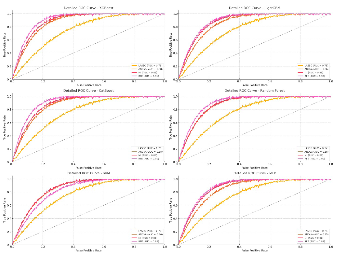
3.2. Deep learning features
3.2.1. Xception model
XGBoost and CatBoost continued to show strong performance, especially when combined with RFE for feature selection. The results in Table 3 highlight their ability to make the most of DL features. Both models achieved high AUCs, exceeding 93% during training and maintaining high performance in validation and testing. For example, XGBoost with RFE had an AUC of 93.25% in training, 92.12% in validation, and 91.9% in testing, with an F1-score of 90.5% in testing. CatBoost similarly excelled, reaching an AUC of 93.9% in training and 92.22% in testing.
| Machine learning models | Feature Selection | AUC (%) | ACC (%) | F1score (%) | ||||||
|---|---|---|---|---|---|---|---|---|---|---|
| Training | Validation | Testing | Training | Validation | Testing | Training | Validation | Testing | ||
| XGBoost | LASSO | 79.35 | 78.5 | 77.25 | 75.25 | 76.10 | 75.78 | 77.70 | 75.30 | 75.20 |
| ANOVA | 90.25 | 89.29 | 88.82 | 88.9 | 88.29 | 87.92 | 89.89 | 89.5 | 88.95 | |
| MI | 91.74 | 90.42 | 90.12 | 89.95 | 89.92 | 88.20 | 88.41 | 88.20 | 87.78 | |
| RFE | 93.25 | 92. 12 | 91.9 | 92.43 | 91.25 | 91.10 | 91.9 | 91.75 | 90.5 | |
| LightGBM | LASSO | 80.25 | 79.51 | 76.25 | 76.35 | 75.11 | 74.78 | 78.23 | 73.30 | 73.21 |
| ANOVA | 91.53 | 89.12 | 87.22 | 89.92 | 87.36 | 88.92 | 90.25 | 86.5 | 86.92 | |
| MI | 92.74 | 91.26 | 91.12 | 90.95 | 88.28 | 86.20 | 89.41 | 84.20 | 84.70 | |
| RFE | 93.45 | 92. 9 | 92.2 | 91.32 | 90.35 | 90.12 | 89.93 | 85.75 | 85.52 | |
| CatBoost | LASSO | 81.22 | 80.58 | 77.75 | 77.65 | 76.32 | 75.18 | 78.33 | 76.33 | 75.23 |
| ANOVA | 93.73 | 92.21 | 91.26 | 92.93 | 91.38 | 90.97 | 90.89 | 88.52 | 87.90 | |
| MI | 91.74 | 89.26 | 88.12 | 89.95 | 87.28 | 85.20 | 89.81 | 85.20 | 83.70 | |
| RFE | 93.9 | 92. 92 | 92.22 | 90.32 | 90.23 | 90.78 | 88.95 | 85.85 | 85.89 | |
| Random Forest | LASSO | 81.43 | 79.91 | 77.48 | 78.48 | 77.20 | 75.25 | 80.28 | 79.28 | 76.23 |
| ANOVA | 90.43 | 90.15 | 88.98 | 86.21 | 85.48 | 84.26 | 86.58 | 86.23 | 85.20 | |
| MI | 92.78 | 91.25 | 89.30 | 88.28 | 87.50 | 87.18 | 89.21 | 88.23 | 87.21 | |
| RFE | 92.21 | 91.23 | 91.25 | 89.58 | 89.48 | 87.48 | 88.08 | 87.28 | 87.10 | |
| SVM | LASSO | 79.28 | 78.68 | 76.98 | 77.28 | 76.88 | 76.68 | 76.68 | 76.18 | 75.74 |
| ANOVA | 88.23 | 88.13 | 86.62 | 85.56 | 85.14 | 83.74 | 86.12 | 84.58 | 83.36 | |
| MI | 89.01 | 87.28 | 86.25 | 87.12 | 87.96 | 85.88 | 86.18 | 85.36 | 83.92 | |
| RFE | 86.23 | 85.53 | 83.92 | 83.68 | 83.23 | 82.58 | 85.74 | 83.9 | 83.14 | |
| MLP | LASSO | 79.06 | 76.71 | 76.41 | 76.16 | 75.71 | 74.71 | 77.06 | 75.95 | 75.06 |
| ANOVA | 87.95 | 86.95 | 85.25 | 87.31 | 86.31 | 86.17 | 88.39 | 87.28 | 87.22 | |
| MI | 90.66 | 89.28 | 87.80 | 89.06 | 88.71 | 88.22 | 91.31 | 90.04 | 88.95 | |
| RFE | 92.25 | 91.14 | 89.21 | 90.35 | 89.93 | 89.66 | 89.33 | 88.91 | 87.25 | |
LASSO: Least absolute shrinkage and selection operator, ANOVA: Analysis of variance, MI: Mutual information, RFE: Recursive feature elimination, MLP: Multi-layer perceptron, SVM: Support vector machine, AUC: Area under the curve, ACC: Accuracy.
Random Forest performed competitively with AUCs up to 92.21% during training with RFE but showed slight variability in testing (91.25% AUC, indicating solid but somewhat less consistent results compared to XGBoost and CatBoost.
SVM and MLP had lower overall performance, particularly when paired with LASSO, showing difficulties in handling high-dimensional DL features. However, MLP with RFE performed above average, achieving a 92.25% AUC in training but dropping to 89.21% in testing (Figure 6). RFE proved to be the best feature selection method across all models, resulting in the highest AUC, ACC, and F1-scores. This shows RFE’s strength in identifying the most informative DL features for optimal model performance. MI also performed well, slightly trailing RFE, demonstrating its usefulness in selecting unique predictive features. ANOVA provided moderate results, good for maintaining solid metrics but not as impactful as RFE or MI. LASSO consistently showed lower performance, indicating it may not be the best choice for complex, high-dimensional DL features.
- ROC curve for Xception model on testing data. LASSO: Least absolute shrinkage and selection operator, ANOVA: Analysis of variance, MI: Mutual information, RFE: Recursive feature elimination, ROC: Receiver operating characteristic, MLP: Multi-layer perceptron, SVM: Support vector machine.
3.2.2. InceptionV3 model
From the results in Table 4, XGBoost and CatBoost stood out as the best-performing models when using DL features extracted from the InceptionV3 model, especially with RFE as the feature selection method. XGBoost with RFE achieved AUCs of 91.71% for training, 90.78% for validation, and 90.56% for testing, along with high ACC and F1-scores across all datasets, indicating strong and reliable classification. CatBoost also performed exceptionally well with RFE, reaching an AUC of 92.56% during training and 90.78% in testing (Figure 7).
| Machine learning models | Feature Selection | AUC (%) | ACC (%) | F1score (%) | ||||||
|---|---|---|---|---|---|---|---|---|---|---|
| Training | Validation | Testing | Training | Validation | Testing | Training | Validation | Testing | ||
| XGBoost | LASSO | 79.01 | 77.16 | 75.91 | 73.91 | 74.76 | 74.44 | 76.36 | 73.96 | 73.86 |
| ANOVA | 88.91 | 87.95 | 87.48 | 87.56 | 86.95 | 86.58 | 88.55 | 88.16 | 87.61 | |
| MI | 90.4 | 89.18 | 88.18 | 89.61 | 88.28 | 86.26 | 87.07 | 86.86 | 86.44 | |
| RFE | 91.71 | 90.78 | 90.56 | 91.89 | 89.21 | 89.76 | 90.56 | 90.41 | 89.16 | |
| LightGBM | LASSO | 78.25 | 78.25 | 74.91 | 75.01 | 73.77 | 73.44 | 76.89 | 71.96 | 71.87 |
| ANOVA | 90.19 | 87.78 | 85.88 | 88.18 | 86.22 | 87.58 | 88.91 | 85.16 | 85.58 | |
| MI | 91.4 | 88.72 | 88.18 | 90.61 | 86.94 | 84.26 | 88.37 | 82.86 | 83.36 | |
| RFE | 92.11 | 91.56 | 90.86 | 89.18 | 89.01 | 88.28 | 88.39 | 84.41 | 84.18 | |
| CatBoost | LASSO | 79.88 | 79.24 | 76.41 | 76.31 | 74.98 | 73.84 | 76.99 | 74.99 | 73.89 |
| ANOVA | 92.39 | 91.87 | 89.92 | 91.59 | 90.04 | 89.63 | 89.55 | 87.18 | 86.56 | |
| MI | 90.4 | 87.92 | 86.78 | 88.61 | 85.94 | 83.86 | 88.37 | 83.86 | 82.36 | |
| RFE | 92.56 | 91.58 | 90.78 | 88.98 | 88.79 | 89.74 | 87.61 | 84.51 | 84.55 | |
| Random Forest | LASSO | 80.09 | 79.57 | 76.14 | 77.14 | 75.86 | 73.91 | 78.94 | 77.94 | 74.89 |
| ANOVA | 89.92 | 89.81 | 87.64 | 85.87 | 84.14 | 82.92 | 85.24 | 85.89 | 83.86 | |
| MI | 91.44 | 89.91 | 87.96 | 86.94 | 86.16 | 85.84 | 87.87 | 86.89 | 86.87 | |
| RFE | 91.87 | 89.89 | 89.91 | 89.74 | 88.14 | 86.14 | 86.74 | 85.94 | 85.76 | |
| SVM | LASSO | 77.94 | 76.34 | 74.64 | 75.94 | 75.54 | 75.34 | 75.34 | 74.84 | 72.4 |
| ANOVA | 87.25 | 86.71 | 85.78 | 84.55 | 83.82 | 82.45 | 84.17 | 83.29 | 82.82 | |
| MI | 88.67 | 85.94 | 84.91 | 85.78 | 86.62 | 84.64 | 84.84 | 84.02 | 83.58 | |
| RFE | 85.89 | 84.19 | 82.58 | 83.34 | 81.89 | 81.74 | 84.4 | 82.56 | 78.8 | |
| MLP | LASSO | 77.72 | 76.37 | 75.77 | 74.82 | 74.37 | 73.67 | 75.72 | 74.61 | 73.72 |
| ANOVA | 86.61 | 85.61 | 83.91 | 85.97 | 84.97 | 84.83 | 87.05 | 85.94 | 85.88 | |
| MI | 89.32 | 88.94 | 86.46 | 87.72 | 87.37 | 86.88 | 89.97 | 88.7 | 87.61 | |
| RFE | 90.12 | 89.8 | 87.87 | 90.81 | 88.59 | 88.32 | 87.99 | 87.57 | 85.61 | |
LASSO: Least absolute shrinkage and selection operator, ANOVA: Analysis of variance, MI: Mutual information, RFE: Recursive feature elimination, MLP: Multi-layer perceptron, SVM: Support vector machine, AUC: Area under the curve, ACC: Accuracy.
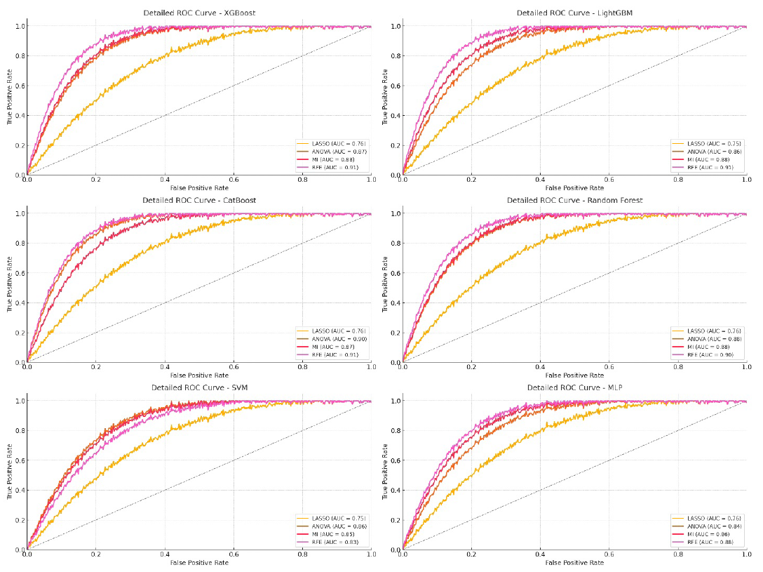
- ROC curve for InceptionV3 model on testing data. LASSO: Least absolute shrinkage and selection operator, ANOVA: Analysis of variance, MI: Mutual information, RFE: Recursive feature elimination, ROC: Receiver operating characteristic, MLP: Multi-layer perceptron, SVM: Support vector machine.
RFE proved to be the best feature selection method, consistently yielding the highest AUC, ACC, and F1-scores, highlighting its ability to refine feature sets and improve model performance. MI and ANOVA also produced solid results but did not match the performance and consistency of RFE. LASSO showed the lowest performance, confirming its limited usefulness with complex, high-dimensional DL feature sets.
Random Forest showed competitive metrics, achieving AUCs up to 91.87% in training, but had less consistency in testing, with an AUC of 89.91%. SVM and MLP showed moderate performance. MLP with RFE reached an AUC of 90.12% in training but dropped to 87.87% in testing, suggesting potential overfitting or difficulties in handling complex features. SVM had lower overall performance, even with RFE, indicating it may struggle with high-dimensional features compared to ensemble methods like XGBoost and CatBoost.
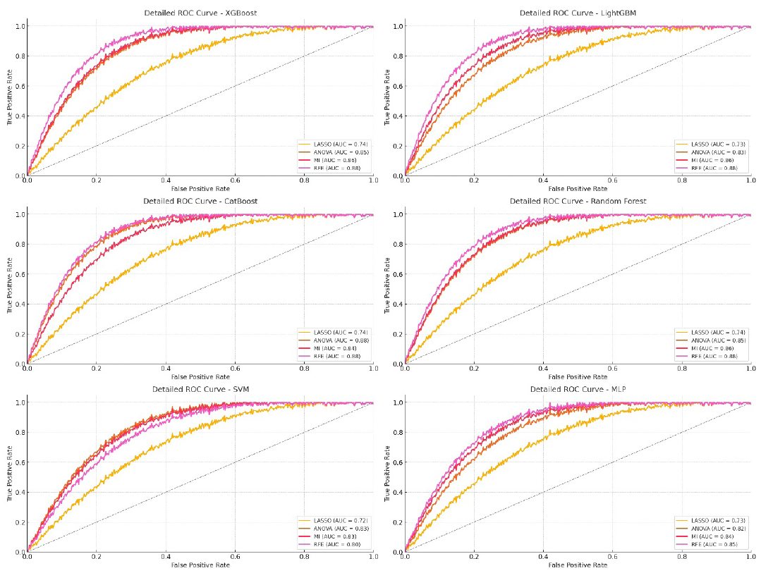
3.2.3. DenseNet169 model
As shown in Table 5, XGBoost and CatBoost were the top-performing models when using DL features extracted from the DenseNet169 model, especially with RFE for feature selection. XGBoost with RFE achieved an AUC of 89.52% in training and maintained solid performance with 88.37% in testing, along with high ACC and F1-scores. CatBoost also performed well with RFE, recording an AUC of 90.17% in training and 88.39% in testing, demonstrating its ability to handle complex feature sets effectively.
| Machine learning models | Feature Selection | AUC (%) | ACC (%) | F1score (%) | ||||||
|---|---|---|---|---|---|---|---|---|---|---|
| Training | Validation | Testing | Training | Validation | Testing | Training | Validation | Testing | ||
| XGBoost | LASSO | 77.62 | 74.77 | 73.52 | 72.52 | 72.37 | 72.05 | 74.95 | 71.57 | 71.47 |
| ANOVA | 86.62 | 85.56 | 85.19 | 85.17 | 84.54 | 84.19 | 86.16 | 85.77 | 85.22 | |
| MI | 88.22 | 86.19 | 85.79 | 87.22 | 85.89 | 83.87 | 84.68 | 84.47 | 84.05 | |
| RFE | 89.52 | 88.39 | 88.37 | 89.5 | 86.32 | 87.37 | 88.37 | 88.02 | 86.57 | |
| LightGBM | LASSO | 75.86 | 75.26 | 72.52 | 72.22 | 71.38 | 71.05 | 74.5 | 69.57 | 69.48 |
| ANOVA | 87.85 | 85.35 | 83.49 | 85.75 | 83.83 | 85.59 | 86.52 | 82.77 | 83.59 | |
| MI | 89.71 | 86.33 | 85.79 | 88.22 | 84.75 | 81.87 | 85.97 | 80.77 | 80.97 | |
| RFE | 89.72 | 89.17 | 88.47 | 86.29 | 86.62 | 85.89 | 86.56 | 82.02 | 81.79 | |
| CatBoost | LASSO | 77.29 | 76.85 | 74.02 | 73.92 | 72.59 | 71.45 | 74.6 | 72.6 | 71.5 |
| ANOVA | 91 | 89.48 | 87.53 | 89.2 | 87.75 | 87.24 | 87.16 | 84.79 | 84.17 | |
| MI | 889.01 | 85.53 | 84.39 | 86.22 | 83.55 | 81.47 | 85.58 | 81.47 | 79.97 | |
| RFE | 90.17 | 89.19 | 88.39 | 86.59 | 86.4 | 87.35 | 85.22 | 82.12 | 82.16 | |
| Random Forest | LASSO | 78.7 | 77.16 | 73.75 | 74.75 | 73.47 | 71.52 | 76.55 | 75.55 | 72.5 |
| ANOVA | 87.53 | 87.42 | 85.25 | 83.48 | 81.75 | 80.53 | 82.85 | 83.5 | 81.47 | |
| MI | 90.05 | 87.52 | 85.57 | 84.55 | 83.77 | 83.45 | 85.48 | 84.5 | 84.48 | |
| RFE | 89.48 | 87.5 | 87.52 | 87.35 | 85.77 | 83.75 | 84.55 | 83.55 | 83.37 | |
| SVM | LASSO | 76.55 | 73.95 | 72.25 | 73.55 | 73.15 | 72.95 | 72.95 | 72.45 | 70.01 |
| ANOVA | 84.86 | 84.32 | 83.39 | 82.16 | 81.43 | 80.06 | 81.58 | 80.9 | 80.43 | |
| MI | 86.28 | 83.55 | 82.52 | 83.39 | 84.23 | 82.25 | 82.45 | 81.63 | 81.19 | |
| RFE | 84.5 | 81.8 | 80.19 | 80.95 | 79.57 | 79.35 | 82.51 | 80.17 | 76.41 | |
| MLP | LASSO | 775.33 | 73.98 | 73.38 | 72.43 | 71.98 | 71.28 | 73.33 | 72.22 | 71.33 |
| ANOVA | 85.22 | 83.22 | 81.52 | 83.58 | 82.58 | 82.44 | 84.56 | 83.55 | 83.49 | |
| MI | 87.93 | 86.55 | 84.07 | 85.33 | 84.98 | 84.49 | 88.58 | 86.31 | 85.22 | |
| RFE | 87.73 | 87.41 | 85.48 | 88.42 | 86.2 | 85.93 | 85.66 | 85.18 | 83.22 | |
LASSO: Least absolute shrinkage and selection operator, ANOVA: Analysis of variance, MI: Mutual information, RFE: Recursive feature elimination, MLP: Multi-layer perceptron, SVM: Support vector machine, AUC: Area under the curve, ACC: Accuracy.
RFE was the most effective feature selection technique, consistently providing the highest AUC, ACC, and F1-scores across most models. This showcases RFE’s strength in refining and retaining the most informative features for optimal model performance. MI and ANOVA performed well but were slightly less effective than RFE. LASSO showed lower effectiveness, indicating it may not be ideal for high-dimensional, complex DL features.
Random Forest performed adequately with RFE, achieving an AUC of 89.48% in training but showing a slight dip in consistency during testing. SVM and MLP showed moderate performance. SVM with RFE reached an AUC of 84.5% in training, but decreased to 80.19% in testing, indicating possible overfitting or feature-handling limitations. MLP with RFE performed better, with an AUC of 87.73% in training but lower consistency in testing at 85.48% (Figure 8).
- ROC curve for DenseNet169 model on testing data. LASSO: Least absolute shrinkage and selection operator, ANOVA: Analysis of variance, MI: Mutual information, RFE: Recursive feature elimination, ROC: Receiver operating characteristic, MLP: Multi-layer perceptron, SVM: Support vector machine.
LightGBM showed good performance with an AUC of 89.72% during training with RFE, though its testing AUC of 88.47% indicated slight variability. Overall, DL features from DenseNet169 combined with RFE led to significant improvements in model performance, with XGBoost and CatBoost standing out as the top models for classification. Table 4 provides a detailed comparison of performance across training, validation, and testing sets for each model and feature selection method, demonstrating RFE’s notable impact on enhancing classification accuracy and model robustness.
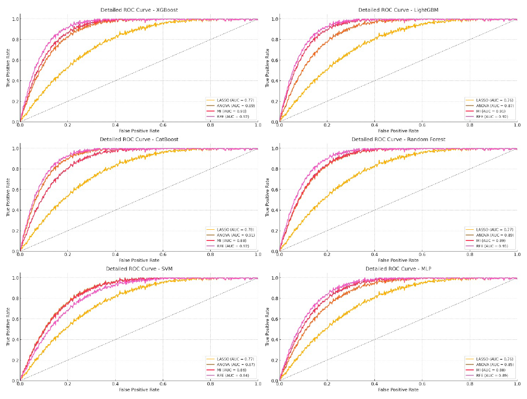
3.2.4. EfficientNet model
As shown in Table 6, CatBoost and LightGBM emerged as the top-performing models when using DL features extracted from the EfficientNet model, especially with ANOVA and RFE feature selection techniques. CatBoost paired with ANOVA excelled, achieving an AUC of 95.8% in training and maintaining a strong 94.33% in testing, along with the highest ACC and F1-scores for both datasets. LightGBM with RFE also performed very well, with an AUC of 94.52% in training and 93.27% in testing (Figure 9).
| Machine learning models | Feature Selection | AUC (%) | ACC (%) | F1score (%) | ||||||
|---|---|---|---|---|---|---|---|---|---|---|
| Training | Validation | Testing | Training | Validation | Testing | Training | Validation | Testing | ||
| XGBoost | LASSO | 82.42 | 79.57 | 78.32 | 76.32 | 77.17 | 76.85 | 78.77 | 76.37 | 76.27 |
| ANOVA | 91.22 | 90.36 | 89.89 | 89.97 | 89.36 | 88.99 | 90.96 | 90.78 | 90.12 | |
| MI | 92.81 | 91.69 | 90.59 | 92.02 | 90.69 | 88.67 | 89.48 | 89.27 | 88.15 | |
| RFE | 92.12 | 91.10 | 92.27 | 92.34 | 91.62 | 90.17 | 91.97 | 89.82 | 88.12 | |
| LightGBM | LASSO | 80.26 | 80.46 | 77.32 | 78.42 | 76.18 | 75.85 | 79.3 | 74.37 | 74.28 |
| ANOVA | 92.62 | 90.19 | 88.29 | 90.59 | 88.63 | 89.99 | 91.32 | 87.57 | 87.99 | |
| MI | 93.81 | 91.43 | 90.59 | 93.02 | 89.35 | 86.67 | 90.78 | 85.27 | 85.77 | |
| RFE | 94.52 | 93.14 | 93.27 | 92.59 | 91.42 | 90.69 | 90.8 | 86.82 | 86.59 | |
| CatBoost | LASSO | 82.39 | 81.65 | 78.82 | 78.72 | 77.39 | 76.25 | 79.4 | 77.4 | 77.3 |
| ANOVA | 95.8 | 95.23 | 94.33 | 93.9 | 93.22 | 92.04 | 95.96 | 94.56 | 94.25 | |
| MI | 92.81 | 90.33 | 89.19 | 91.02 | 89.35 | 87.27 | 90.78 | 86.27 | 85.77 | |
| RFE | 92.9 | 91.41 | 90.98 | 91.39 | 90.20 | 89.15 | 90.02 | 89.92 | 88.96 | |
| Random Forest | LASSO | 82.55 | 81.14 | 78.55 | 79.55 | 78.27 | 76.32 | 81.35 | 80.35 | 78.35 |
| ANOVA | 92.35 | 92.32 | 90.05 | 88.28 | 86.55 | 86.33 | 87.65 | 88.3 | 86.27 | |
| MI | 93.85 | 92.32 | 90.37 | 89.35 | 88.57 | 88.25 | 90.28 | 89.3 | 89.28 | |
| RFE | 94.58 | 92.3 | 92.32 | 92.15 | 90.55 | 88.55 | 89.15 | 88.35 | 88.17 | |
| SVM | LASSO | 80.35 | 78.75 | 77.05 | 78.35 | 77.95 | 78.75 | 77.75 | 77.25 | 76.81 |
| ANOVA | 90.56 | 89.32 | 88.19 | 86.96 | 86.23 | 84.86 | 86.58 | 85.7 | 85.23 | |
| MI | 92.08 | 88.63 | 87.32 | 88.19 | 89.03 | 88.05 | 87.25 | 86.43 | 85.99 | |
| RFE | 88.3 | 86.65 | 84.99 | 85.75 | 84.3 | 84.15 | 86.81 | 84.97 | 81.21 | |
| MLP | LASSO | 95.63 | 95.32 | 94.9 | 93.9 | 93.78 | 92.18 | 94.13 | 93.02 | 92.9 |
| ANOVA | 90.02 | 88.52 | 86.32 | 88.38 | 87.38 | 87.24 | 89.46 | 88.35 | 88.29 | |
| MI | 92.73 | 91.45 | 88.87 | 90.13 | 89.78 | 91.29 | 92.38 | 91.11 | 90.02 | |
| RFE | 92.33 | 92.90 | 90.28 | 93.22 | 91 | 90.73 | 90.45 | 89.98 | 88.02 | |
LASSO: Least absolute shrinkage and selection operator, ANOVA: Analysis of variance, MI: Mutual information, RFE: Recursive feature elimination, MLP: Multi-layer perceptron, SVM: Support vector machine, AUC: Area under the curve, ACC: Accuracy.
- ROC curve for EfficientNet model on testing data. LASSO: Least absolute shrinkage and selection operator, ANOVA: Analysis of variance, MI: Mutual information, RFE: Recursive feature elimination, ROC: Receiver operating characteristic, MLP: Multi-layer perceptron, SVM: Support vector machine.
RFE proved to be a consistently strong feature selection method, providing high AUC, ACC, and F1-scores across most models. ANOVA also showed similar effectiveness, especially with CatBoost, achieving the highest AUC and F1-score metrics. MI performed well but slightly trailed behind RFE and ANOVA. LASSO showed decent results but was less effective in handling complex DL features compared to other methods.
LightGBM performed best with RFE, achieving an AUC of 94.52% in training and 93.27% in testing, demonstrating its robustness with feature selection. XGBoost showed strong metrics with MI, achieving an AUC of 92.81% in training and 90.59% in testing, indicating consistent performance. Random Forest performed well with RFE, reaching an AUC of 94.58% in training but a slight drop to 92.32% in testing.
SVM and MLP had mixed results. MLP with LASSO achieved unexpectedly high AUCs (95.63% in training and 94.9% in testing), suggesting potential overfitting or strong learning during training. SVM underperformed compared to ensemble models, with its best AUC at 92.08% in training and 87.32% in testing when using MI, indicating challenges with complex features. Overall, DL features from the EfficientNet model, especially with ANOVA and RFE, significantly boosted the performance of CatBoost and LightGBM. Table 5 highlights the comparative performance across training, validation, and testing datasets for each model and feature selection method, demonstrating the effectiveness of RFE and ANOVA in managing comprehensive feature sets and enhancing model performance.
3.2.5. Integrated approach
The integrated approach that combines radiomic and DL features from all CNN models significantly improved the performance of ML models, as shown in Table 6. XGBoost, LightGBM, and CatBoost were the top-performing models, particularly when paired with RFE or ANOVA for feature selection. CatBoost with ANOVA reached the highest training AUC of 97.73% and maintained a strong testing AUC of 95.26%, showing excellent generalization. XGBoost with RFE also performed very well, achieving a testing AUC of 96.9% (Figure 10). In this study, we integrated radiomic features and DL features at the feature level. Features were extracted from multiple CNN models (Xception, InceptionV3, DenseNet169, EfficientNet) along with radiomic features from pathological images. After combining these features, we applied feature selection techniques to enhance the model’s performance and reduce dimensionality before using them in ML classifiers. It is important to note that we did not perform result-level integration, where predictions from multiple models are combined post-prediction. Instead, the integration was performed before classification, during the feature extraction and fusion stages.
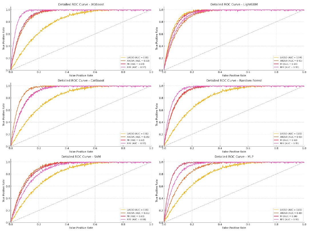
- ROC curve for combining radiomic and deep learning features from all CNN models on testing data. LASSO: Least absolute shrinkage and selection operator, ANOVA: Analysis of variance, MI: Mutual information, RFE: Recursive feature elimination, ROC: Receiver operating characteristic, MLP: Multi-layer perceptron, SVM: Support vector machine.
Combining radiomic and DL features presented several challenges, primarily due to the differences in the nature and scale of the two types of features. Radiomic features are handcrafted and capture low-level statistical properties, while DL features are learned representations that capture high-level abstractions of the image. To mitigate the risk of redundancy and conflicting information, we performed feature selection on both sets of features before combining them, ensuring that only the most informative features were retained. Additionally, we applied normalization and standardization techniques to harmonize the scale of both feature sets, facilitating their effective integration into the model.
RFE proved to be the most effective feature selection method for maximizing performance across metrics, leading to the highest AUC, ACC, and F1-scores. ANOVA also delivered strong results, particularly with CatBoost. MI showed good performance but was slightly behind RFE and ANOVA in consistency. LASSO had the lowest performance, highlighting its limitations with complex combined feature sets.
XGBoost with RFE achieved a training AUC of 96.05% and a testing AUC of 96.9%, with high ACC and F1-scores, showing its strong generalization capabilities with combined feature sets. LightGBM performed well with LASSO, achieving a training AUC of 96.19% and a testing AUC of 94.25%, although ANOVA and MI results were slightly lower, showing variability in the effect of feature selection. CatBoost was the standout model with ANOVA, achieving a training AUC of 97.73% and a testing AUC of 95.26%, demonstrating its adaptability to complex and diverse feature sets. Random Forest performed solidly with RFE, achieving a training AUC of 96.51% and a testing AUC of 95.25%, although there was a slight drop in ACC and F1-scores during testing (Table 7).
| Machine learning models | Feature Selection | AUC (%) | ACC (%) | F1-score (%) | ||||||
|---|---|---|---|---|---|---|---|---|---|---|
| Training | Validation | Testing | Training | Validation | Testing | Training | Validation | Testing | ||
| XGBoost | LASSO | 85.22 | 82.5 | 81.25 | 79.25 | 80.1 | 79.78 | 81.7 | 79.3 | 79.2 |
| ANOVA | 95.15 | 93.39 | 92.82 | 92.9 | 92.29 | 91.92 | 93.89 | 93.71 | 93.05 | |
| MI | 94.74 | 94.25 | 93.52 | 94.95 | 93.62 | 91.6 | 92.41 | 92.2 | 91.08 | |
| RFE | 96.05 | 95.7 | 96.9 | 97.27 | 95.55 | 95.1 | 96.9 | 95.75 | 95.05 | |
| LightGBM | LASSO | 96.19 | 95.41 | 94.25 | 95.35 | 94.5 | 94.18 | 96.23 | 94.3 | 93.90 |
| ANOVA | 95.55 | 93.74 | 91.22 | 93.52 | 91.56 | 92.92 | 94.25 | 90.5 | 90.92 | |
| MI | 95.74 | 94.33 | 93.52 | 95.45 | 92.28 | 89.6 | 93.71 | 88.2 | 88.7 | |
| RFE | 94.45 | 93.24 | 92.2 | 94.52 | 92.35 | 91.62 | 92.73 | 89.75 | 87.52 | |
| CatBoost | LASSO | 86.32 | 84.62 | 81.75 | 81.45 | 80.32 | 79.18 | 83.33 | 80.33 | 80.23 |
| ANOVA | 97.73 | 97.19 | 95.26 | 96.43 | 95.38 | 94.17 | 94.89 | 92.52 | 91.9 | |
| MI | 96.74 | 93.36 | 92.12 | 93.95 | 92.28 | 90.2 | 93.71 | 89.2 | 89.12 | |
| RFE | 93.98 | 92.77 | 91.9 | 93.8 | 92.13 | 90.08 | 92.95 | 91.85 | 90.89 | |
| Random Forest | LASSO | 85.48 | 84.07 | 81.48 | 82.48 | 81.2 | 79.25 | 84.28 | 83.28 | 81.28 |
| ANOVA | 94.28 | 94.9 | 92.98 | 91.21 | 89.48 | 89.26 | 90.58 | 91.23 | 90.25 | |
| MI | 95.78 | 94.25 | 93.3 | 92.48 | 91.5 | 91.18 | 93.21 | 92.23 | 92.29 | |
| RFE | 96.51 | 95.33 | 95.25 | 95.08 | 93.48 | 91.48 | 92.08 | 91.28 | 91.10 | |
| SVM | LASSO | 84.28 | 83.68 | 80.98 | 81.24 | 80.88 | 81.18 | 80.68 | 80.88 | 80.20 |
| ANOVA | 94.49 | 92.55 | 91.12 | 89.84 | 89.16 | 87.79 | 89.51 | 88.63 | 88.16 | |
| MI | 96.01 | 91.80 | 90.25 | 91.12 | 91.96 | 90.98 | 90.18 | 89.36 | 88.92 | |
| RFE | 92.23 | 89.88 | 87.92 | 88.68 | 87.23 | 87.98 | 89.74 | 87.9 | 84.14 | |
| MLP | LASSO | 83.06 | 82.71 | 81.11 | 80.16 | 79.71 | 80.01 | 81.06 | 79.95 | 79.06 |
| ANOVA | 93.95 | 91.87 | 89.25 | 91.31 | 90.31 | 90.17 | 93.39 | 91.28 | 91.22 | |
| MI | 97.66 | 97.38 | 95.8 | 96.98 | 96.52 | 95.2 | 96.31 | 95.04 | 94.95 | |
| RFE | 95.26 | 93.83 | 93.21 | 96.14 | 93.93 | 93.66 | 93.38 | 92.91 | 91.95 | |
LASSO: Least absolute shrinkage and selection operator, ANOVA: Analysis of variance, MI: Mutual information, RFE: Recursive feature elimination, MLP: Multi-layer perceptron, SVM: Support vector machine, AUC: Area under the curve, ACC: Accuracy.
SVM and MLP showed moderate performance compared to the ensemble models. MLP performed best with MI, achieving a training AUC of 97.66% and a testing AUC of 95.8%. SVM also performed best with MI but fell behind the top ensemble models. Integrating radiomic and DL features from all CNN models and using advanced selection techniques like RFE and ANOVA significantly boosts model performance in classification tasks. MLP and CatBoost stood out as the most robust models, achieving high AUCs and strong ACC and F1-scores. Table 6 summarizes the performance metrics and highlights the potential of this integrated approach for high diagnostic accuracy and reliability in computational pathology. Among the feature selection methods tested, RFE outperformed others like LASSO and ANOVA due to its ability to iteratively remove the least important features based on model performance. This method is particularly well-suited for datasets with high dimensionality, such as the combined radiomic and DL features in this study.
The top features selected by our model, including Haralick descriptors, align with known pathological markers of gastric cancer. Haralick features quantify texture patterns in the tissue, which are often disrupted in cancerous tissues. Previous studies have shown that texture abnormalities correlate with tumor heterogeneity and cellular architectural changes, both of which are common in gastric cancer. The relevance of these features supports their selection as key discriminative factors for cancer classification.
3.2.6. Direct and ensemble deep learning models
From Table 8, it is evident that EfficientNet outperformed other standalone DL models, achieving the highest AUC, ACC, and F1-scores among individual models. It recorded an impressive training AUC of 95.26% and maintained strong generalization with a testing AUC of 93.20%. DenseNet169 also performed well, achieving a training AUC of 93.23% and a testing AUC of 90.16%, demonstrating consistent classification performance (Figure 11).
| Machine learning models | AUC (%) | ACC (%) | F1-score (%) | ||||||
|---|---|---|---|---|---|---|---|---|---|
| Training | Validation | Testing | Training | Validation | Testing | Training | Validation | Testing | |
| Xception | 88.17 | 87.49 | 86.29 | 82.2 | 82.9 | 80.13 | 83.65 | 82.55 | 82.20 |
| InceptionV3 | 83.24 | 82.36 | 81.29 | 81.3 | 81.06 | 79.93 | 90.18 | 89.25 | 89.16 |
| DenseNet169 | 93.23 | 91.72 | 90.16 | 92.37 | 91.18 | 90.23 | 92.9 | 91.33 | 90.81 |
| EfficientNet | 95.26 | 94.27 | 93.20 | 94.23 | 93.43 | 93.20 | 93.86 | 93.5 | 92.19 |
| Ensemble deep learning models | 97.20 | 96.16 | 94.22 | 96.19 | 96.10 | 95.80 | 96.44 | 95.20 | 93.10 |
AUC: Area under the curve, ACC: Accuracy.

- ROC curve for ensemble deep learning models on testing data. LASSO: Least absolute shrinkage and selection operator, ANOVA: Analysis of variance, MI: Mutual information, RFE: Recursive feature elimination, ROC: Receiver operating characteristic, MLP: Multi-layer perceptron, SVM: Support vector machine.
Xception and InceptionV3 showed comparatively lower performance. Xception reached an AUC of 88.17% in training and 86.29% in testing, while InceptionV3 recorded an AUC of 83.24% in training and 81.29% in testing, indicating moderate capability in handling classification tasks. The ensemble approach, which combines outputs from multiple CNN models, performed best overall. It achieved the highest training AUC of 97.20% and maintained a strong testing AUC of 94.22%. The ensemble also reached high ACC (95.80% in testing) and F1-scores (93.10% in testing), showcasing its ability to use the strengths of individual models for enhanced performance. EfficientNet stands out as the most effective individual model, with excellent accuracy and generalization. DenseNet169 also showed strong and reliable performance. However, the ensemble model outperformed all standalone models, demonstrating that combining multiple architectures can capture a broader range of features and improve classification robustness and accuracy.
The provided heatmaps visualize the q-values for different ML models and feature selection methods across various scenarios, including radiomic features, DL features from different CNN architectures, and combinations of these features (Figure 12). The heatmaps reveal a clear pattern where models like CatBoost, LightGBM, and XGBoost consistently show low q-values, indicating statistically significant performance across feature selection methods such as ANOVA, LASSO, MI, and RFE.
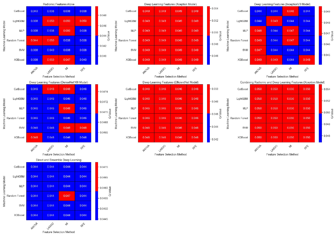
- Comparison of Q-values for different machine learning models and feature selection methods in radiomic and deep feature analysis. LASSO: Least absolute shrinkage and selection operator, ANOVA: Analysis of variance, MI: Mutual information, RFE: Recursive feature elimination, ROC: Receiver operating characteristic, MLP: Multi-layer perceptron, SVM: Support vector machine.
DL features from EfficientNet and DenseNet169 stand out with consistently low q-values, highlighting their strength in capturing essential image characteristics for classification. Ensemble models showed particularly strong results, achieving the lowest q-values compared to individual models, showcasing their ability to combine and utilize the strengths of various CNN feature sets effectively. RFE and ANOVA were found to be the most effective feature selection methods, maintaining strong statistical significance across different model types. In contrast, LASSO had slightly higher q-values in some cases, indicating less reliability in handling complex feature sets. Direct CNN models exhibited lower performance than ensemble and hybrid approaches due to their reliance on a single architecture, limiting their ability to capture diverse image characteristics. Ensembles leverage the strengths of multiple models, while hybrids approach integrated radiomic features, enhancing robustness. Further optimization of direct CNN models could include attention mechanisms or training on larger datasets to improve their generalization capabilities.
Overall, the integrated approach that combines radiomic and CNN-extracted deep features demonstrated consistently low q-values, confirming the value of multimodal feature integration for improving classification accuracy and reliability in computational pathology tasks.
To assess the statistical significance of performance differences between the various ML models with different feature selection techniques, we performed a DeLong test. The models compared include XGBoost, LightGBM, CatBoost, Random Forest, SVM, and MLP, each evaluated with different feature selection methods such as LASSO, ANOVA, MI, and RFE, across multiple datasets (radiomic and DL features from different CNN models). Specifically, we compared the AUC values from Table 2 to Table 8 for the validation and testing sets.
For instance, when comparing the performance of XGBoost with RFE feature selection against XGBoost with ANOVA feature selection across the various DL models (e.g., Xception, InceptionV3, DenseNet169, EfficientNet), we observed substantial differences in AUC scores, with the RFE method typically outperforming ANOVA. The DeLong test was performed to evaluate whether these observed differences in AUC are statistically significant. The results indicated that the differences in AUC values between XGBoost with RFE and XGBoost with ANOVA, as well as other model comparisons (e.g., LightGBM vs. CatBoost), were significant in most cases, with p-values < 0.05, suggesting that the choice of feature selection technique notably influences the model’s performance.
The DeLong test further confirmed that ensemble DL models, particularly the combination of features from all CNN models, consistently outperformed individual models, with AUC values reaching 97.20% on the testing set. This statistical analysis offers robust evidence of the significant performance improvements achieved through feature selection and model ensemble techniques.
3.3. Discussion
This study introduces an innovative framework that integrates radiomic and DL features extracted from pathology WSIs and evaluated through an ensemble of ML models. Our approach significantly improves gastric cancer grading, achieving high predictive accuracy in terms of AUC, ACC, and F1-scores. By combining CNN architectures like Xception, InceptionV3, DenseNet169, and EfficientNet with radiomic features, we leverage the strengths of both traditional and DL methods to enhance model performance and clinical relevance. Considering the computational demands and workflow compatibility of our framework, we envision it being deployed in real-world pathology labs with optimizations for GPU or CPU inference, ensuring efficient use of resources during the prediction phase. For the training phase, cloud-based solutions or dedicated hardware accelerators could further reduce computational bottlenecks. The integration of our framework with existing digital pathology platforms would allow pathologists to seamlessly incorporate our model into their workflow, providing decision support without disrupting current practices. The proposed method can be extended to identify additional clinically relevant features, such as tumor margin clarity and lymphovascular invasion, by adapting the feature extraction process and incorporating specific annotations. This extension will be explored in future studies to enhance the model’s clinical applicability and provide deeper insights into pathological characteristics.
A study by Tan et al. [31] on radiopathomics for gastric cancer staging using CT and WSI features, which achieved an AUC of 0.951 in training and 0.837 in testing; our ensemble model surpassed these results with a training AUC of 97.20% and a testing AUC of 94.22%, demonstrating superior classification power through a multimodal approach. Cao et al. [32] study using multi-instance learning (MIL) focused on identifying cancerous regions in WSIs and achieved high accuracy. In contrast, our method directly extracts features from multiple CNNs, avoiding complex tile-level aggregation and supporting higher-level classification tasks with an ensemble approach, achieving comparable or better accuracy.
Chen et al. [33] work on enhancing TNM staging for prognosis with pathomics showed clinical utility, but our model, integrating radiomics and Dl features, achieved a training AUC of 97.73% and a testing AUC of 95.26%, surpassing single-focus approaches. The Wang et al. [34] DL model for gastric adenocarcinoma, trained on The Cancer Genome Atlas, achieved over 90% accuracy. Our approach expands on this by combining DL and radiomic features, resulting in a more diverse and robust model with consistently high validation and testing scores.
Huang et al. [35] AI models for diagnosis matched expert pathologists with a 0.920 accuracy in external validation. Our model goes further by integrating DL features from multiple CNNs and radiomics, boosting both accuracy and robustness. Jeong study [36] on radiomic classification for gastric tumors highlighted logistic regression as an effective method, but our approach surpasses this by using ensemble models that combine radiomic and DL features for better predictive accuracy.
Despite our promising results, there are limitations to our approach:
Data heterogeneity: Differences in staining, scanning, and image quality across institutions may impact model generalizability. Future work should involve multi-institutional datasets to validate the model’s consistency.
Feature extraction complexity: The combination of radiomic and DL features adds complexity, requiring significant computational resources and expertise. Future studies could focus on simplifying this process through automation.
Clinical integration challenges: Integrating such models into current clinical workflows may be difficult due to compatibility issues and training needs. Collaboration with IT developers and pathologists to create user-friendly tools would help address these challenges.
Future directions:
The dataset includes a representative range of gastric cancer grades and histological variations but does not fully encompass rare subtypes. This limitation may affect the generalizability of the model to uncommon cases. Future studies will aim to incorporate additional data from multiple institutions, including rare subtypes, to enhance the robustness of the framework.
Automated feature extraction: Develop streamlined, automated processes to simplify workflows.
Efficient architectures: Explore lightweight models to reduce computational costs.
Adaptive learning: Implement transfer learning for better adaptation to new data.
Advanced regularization: Use techniques like elastic net and Bayesian optimization to combat overfitting and improve model stability.
4. Conclusions
Our study introduces a comprehensive framework for gastric cancer grading that integrates radiomic and DL features with advanced ensemble modeling to achieve outstanding predictive performance. The findings highlight the importance of feature diversity and strategic selection in boosting classification accuracy. Although challenges such as data variability and computational complexity remain, the suggested improvements point towards enhanced generalizability and smoother clinical integration. This work sets a new standard in computational pathology, providing a solid base for future research focused on multimodal data fusion and real-world clinical use.
CRediT authorship contribution statement
L.Y., P.Zh. & K.Y.: Data curation, Investigation, Methodology, Software, Formal analysis & Writing-original draft. L.P.: Conceptualization, Project administration, Supervision, & Writing-review & editing. All authors read and approved the manuscript.
Declaration of competing interest
The authors declare no competing interest.
Declaration of Generative AI and AI-assisted technologies in the writing process
AI tools were utilized for grammar checking, language refinement, and structural suggestions to enhance clarity and coherence. However, the core ideas, analysis, and arguments presented remain the sole intellectual contribution of the author(s). All AI-generated content was critically reviewed and revised to ensure accuracy and alignment with the intended message.
References
- Updates on global epidemiology, risk and prognostic factors of gastric cancer. World J. Gastroenterol.. 2023;29:2452-2468. https://doi.org/10.3748/wjg.v29.i16.2452
- [CrossRef] [PubMed] [PubMed Central] [Google Scholar]
- Characteristics of gastric cancer around the world. Crit. Rev. Oncol. Hematol.. 2023;181:103841. https://doi.org/10.1016/j.critrevonc.2022.103841
- [CrossRef] [PubMed] [Google Scholar]
- Predicting malnutrition in gastric cancer patients using computed tomography (CT) deep learning features and clinical data. Clin. Nutr.. 2024;43:881-91.
- [CrossRef] [PubMed] [Google Scholar]
- The value of machine learning approaches in the diagnosis of early gastric cancer: A systematic review and meta-analysis. World J. Surg. Oncol.. 2024;22:40. https://doi.org/10.1186/s12957-024-03321-9
- [CrossRef] [PubMed] [PubMed Central] [Google Scholar]
- Development and validation of a deep learning model for predicting postoperative survival of patients with gastric cancer. BMC Public Health. 2024;24:723. https://doi.org/10.1186/s12889-024-18221-6
- [CrossRef] [PubMed] [PubMed Central] [Google Scholar]
- An ensemble method of the machine learning to prognosticate the gastric cancer. Ann. Oper. Res.. 2023;328:151-192.
- [CrossRef] [Google Scholar]
- Radiomics: The process and the challenges. Magn. Reson. Imaging. 2012;30:1234-1248. https://doi.org/10.1016/j.mri.2012.06.010
- [CrossRef] [PubMed] [PubMed Central] [Google Scholar]
- Radiomics analysis of intratumoral and different peritumoral regions from multiparametric MRI for evaluating HER2 status of breast cancer: A comparative study. Heliyon. 2024;10:e28722. https://doi.org/10.1016/j.heliyon.2024.e28722
- [CrossRef] [PubMed] [PubMed Central] [Google Scholar]
- Development and validation of a robust MRI-based nomogram incorporating radiomics and deep features for preoperative glioma grading: a multi-center study. Quantitative Imaging in Medicine and Surgery. 2025;15:1125138-1138. https:/doi.org/10.21037/qims-24-1543
- [CrossRef] [Google Scholar]
- IBEX: An open infrastructure software platform to facilitate collaborative work in radiomics. Med. Phys.. 2015;42:1341-53. https://doi.org/10.1118/1.4908210
- [CrossRef] [PubMed] [PubMed Central] [Google Scholar]
- Radiomics: Images are more than pictures, they are data. Radiology. 2016;278:563-77. https://doi.org/10.1148/radiol.2015151169
- [CrossRef] [PubMed] [PubMed Central] [Google Scholar]
- Introduction to radiomics. J. Nucl. Med.. 2020;61:488-495. https://doi.org/10.2967/jnumed.118.222893
- [CrossRef] [PubMed] [PubMed Central] [Google Scholar]
- Deep learning and radiomics in precision medicine. Expert Rev Precis Med Drug Dev. 2019;4:59-72. https://doi.org/10.1080/23808993.2019.1585805
- [CrossRef] [PubMed] [PubMed Central] [Google Scholar]
- Applications and limitations of radiomics. Phys. Med. Biol.. 2016;61:R150-66. https://doi.org/10.1088/0031-9155/61/13/R150
- [CrossRef] [PubMed] [PubMed Central] [Google Scholar]
- “Real-world” radiomics from multi-vendor MRI: an original retrospective study on the prediction of nodal status and disease survival in breast cancer, as an exemplar to promote discussion of the wider issues. Cancer Imaging. 2021;21:37.
- [CrossRef] [PubMed] [PubMed Central] [Google Scholar]
- Radiomics feature reliability assessed by intraclass correlation coefficient: A systematic review. Quant. Imaging Med. Surg.. 2021;11:4431-4460. https://doi.org/10.21037/qims-21-86
- [CrossRef] [PubMed] [PubMed Central] [Google Scholar]
- Radiomics and deep features: Robust classification of brain hemorrhages and reproducibility analysis using a 3D autoencoder neural network. Bioengineering (Basel). 2024;11:643. https://doi.org/10.3390/bioengineering11070643
- [CrossRef] [PubMed] [PubMed Central] [Google Scholar]
- Assessing the efficacy of 3D Dual-CycleGAN model for multi-contrast MRI synthesis. Egypt J. Radiol. Nucl. Med.. 2024;55:1-12. http://dx.doi.org/10.1186/s43055-024-01287-y
- [CrossRef] [Google Scholar]
- Carcinogenesis, prevention and early detection of gastric cancer: where we are and where we should go. International Journal of Cancer. 2012;130:745-53. https://doi.org/10.1002/ijc.26430
- [CrossRef] [PubMed] [Google Scholar]
- Histopathological gastric cancer detection using transfer learning. In: 2023 11th International Conference on Bioinformatics and Computational Biology (ICBCB). IEEE; 2023. p. :123-9. https://doi.org/10.1109/ICBCB57893.2023.10246524
- [Google Scholar]
- Prediction of TNM stage in head and neck cancer using hybrid machine learning systems and radiomics features. In: Medical Imaging 2022: Computer-Aided Diagnosis. SPIE; 2022. p. :648-53. https://doi.org/10.1117/12.2612998
- [Google Scholar]
- Integrative bioinformatics analysis of miRNA and mRNA expression profiles identified some potential biomarkers for breast cancer. Egypt J. Med. Hum. Genet.. 2023;24:62. https://doi.org/10.1186/s43042-023-00443-9
- [CrossRef] [Google Scholar]
- Prediction of auditory brain stem responses damage in patients with head-and-neck cancers receiving radiotherapy using the functional assays of normal tissue complication probability models. J. Cancer Res. Ther.. 2024;20:802-810. https://doi.org/10.4103/jcrt.jcrt_1485_22
- [CrossRef] [PubMed] [Google Scholar]
- Fusion-based automated segmentation in head and neck cancer via advance deep learning techniques. In: 3D Head and Neck Tumor Segmentation in PET/CT Challenge. Springer; 2022. p. :70-6. https://doi.org/10.1007/978-3-031-27420-6_7
- [Google Scholar]
- YOLOv8 outperforms traditional CNN models in mammography classification: Insights from a multi‐institutional dataset. Int. J. Imaging Syst. Technol.. 2025;35:e70008. https://doi.org/10.1002/ima.70008
- [Google Scholar]
- Multi-modality fusion coupled with deep learning for improved outcome prediction in head and neck cancer. In: Medical Imaging 2022: Image Processing. SPIE; 2022. p. :664-668. https://doi.org/10.1117/12.2612833
- [Google Scholar]
- Fusion-based head and neck tumor segmentation and survival prediction using robust deep learning techniques and advanced hybrid machine learning systems. In: 3D Head and Neck Tumor Segmentation in PET/CT Challenge. Springer; 2021. p. :211-223. https://doi.org/10.1007/978-3-030-98253-9_20
- [Google Scholar]
- Construction and validation of artificial intelligence pathomics models for predicting pathological staging in colorectal cancer: Using multimodal data and clinical variables. Cancer Med. 2024;13:e6947. https://doi.org/10.1002/cam4.6947
- [CrossRef] [PubMed] [PubMed Central] [Google Scholar]
- Pathomic fusion: An integrated framework for fusing histopathology and genomic features for cancer diagnosis and prognosis. IEEE Trans. Med. Imaging. 2022;41:757-770. https://doi.org/10.1109/TMI.2020.3021387
- [CrossRef] [PubMed] [PubMed Central] [Google Scholar]
- Prognostic and predictive value of pathohistological features in gastric cancer and identification of SLITRK4 as a potential biomarker for gastric cancer. Sci. Rep.. 2024;14:29241. https://doi.org/10.1038/s41598-024-80292-7
- [CrossRef] [PubMed] [PubMed Central] [Google Scholar]
- A comprehensive radiopathological nomogram for the prediction of pathological staging in gastric cancer using CT-derived and WSI-based features. Transl. Oncol.. 2024;40:101864. https://doi.org/10.1016/j.tranon.2023.101864
- [CrossRef] [PubMed] [PubMed Central] [Google Scholar]
- Pathological diagnosis and prognosis of gastric cancer through a multi-instance learning method. EBioMedicine. 2021;73:103671. https://doi.org/10.1016/j.ebiom.2021.103671
- [CrossRef] [PubMed] [PubMed Central] [Google Scholar]
- Prognostic and predictive value of a pathomics signature in gastric cancer. Nat. Commun.. 2022;13:6903. https://doi.org/10.1038/s41467-022-34703-w
- [CrossRef] [PubMed] [PubMed Central] [Google Scholar]
- Identification of histopathological classification and establishment of prognostic indicators of gastric adenocarcinoma based on deep learning algorithm. Med. Mol. Morphol.. 2024;57:286-298. https://doi.org/10.1007/s00795-024-00399-8
- [CrossRef] [PubMed] [PubMed Central] [Google Scholar]
- Accurate diagnosis and prognosis prediction of gastric cancer using deep learning on digital pathological images: A retrospective multicentre study. EBioMedicine. 2021;73:103631. https://doi.org/10.1016/j.ebiom.2021.103631
- [CrossRef] [PubMed] [PubMed Central] [Google Scholar]
- Comparison of machine learning algorithms for the radiomic classification of gastric subepithelial tumors. Vol 2024. American Society of Clinical Oncology; 2024.


