

Translate this page into:
On entropy measures of molecular graphs using topological indices
⁎Corresponding author. shazman724@gmail.com (Shazia Manzoor),
-
Received: ,
Accepted: ,
This article was originally published by Elsevier and was migrated to Scientific Scholar after the change of Publisher.
Peer review under responsibility of King Saud University.
Abstract
Topological indices as a molecular descriptors are important tools in / studies. The graph entropies with topological indices inspired by Shannon’s entropy concept become the information-theoretic quantities for measuring the structural information of chemical graphs and complex networks. The graph entropy measures are playing an important role in a variety of problem areas including, discrete mathematics, biology, and chemistry. Our contribution is to explore graph entropies that are based on a novel information functional, which is the number of vertices of different degree together with the number of edges between different degree vertices.
In this paper, we study the chemical graph of crystal structure of titanium difluoride and crystallographic structure of cuprite . Also, we compute entropies of these structures by making a relation of degree based topological indices namely first redefined Zagreb index, second redefined Zagreb index, third redefined Zagreb index, fourth Atom Bond Connectivity index, fifth Geometric Arithmetic index, Sanskruti index with the help of information function.
Keywords
Entropy
Zagreb type indices
Fourth Atom Bond Connectivity index
Fifth Geometric Arithmetic index
Sanskruti index
Titanium difluoride
Cuprite

1 Introduction
Graph theory plays an important role in modeling and designing any chemical network. A large number of properties like physico-chemical properties, thermodynamic properties, chemical activity and biological activity are determined by the chemical applications of graph theory. These properties can be characterized by certain graph invariants referred to as topological indices. In chemical graph theory, molecular graph is a simple finite graph in which vertices denote the atoms and edges denote the chemical bonds in underlying chemical structure. The topological index is a numeric value or a sequence for a given structure under discussion, which actually shows the physical, chemical and biological properties of graph.
Chemical graph theory is a branch of mathematical chemistry in which tools of graph theory are applied to model the chemical phenomenon mathematically. Also, it relates to the nontrivial applications of graph theory for solving molecular problems. This theory contributes a prominent role in the field of chemical sciences, see for details (Gao et al., 2018). Also Chem-informatics is new subject which is a combination of chemistry, mathematics and information science. It examines Quantitative structure-activity relationship and Quantitative Structure-Property Relationship that are utilized to predict the bioactivity and physiochemical properties of chemical compounds (Wu et al., 2015).
Let G be a graph with be the vertex set and be the edge set of G. The degree of a vertex r is the number of edges of G incident with vertex r. The length of a shortest path in a graph G is a distance between r and s. If G is a graph with p vertices and q edges, then we say the order of G is p and the size of G is q. A graph of order p and size q is addressed as -graph.
In chemical graph, the vertices represent atoms and edges refer as the chemical bonds in underlying chemical structure. A topological index is a numerical value that is computed mathematically from the molecular graph. It is associated with chemical constitution indicating for correlation of chemical structure with many physical, chemical properties and biological activities. The exact formulas of topological indices for chemical graphs have been computed in (Siddiqui et al., 2016; Siddiqui et al., 2016). For further detail of application point see (Gao et al., 2017; Imran et al., 2018).
The concept of entropy was introduced first in Shannon’s famous paper (Shannon, 1948) as “ The entropy of a probability distribution is known as a measure of the unpredictability of information content or a measure of the uncertainty of a system”. Later, entropy was initiated to be applied to graphs nd chemical networks. It was developed for measuring the structural information of graphs and chemical networks. In 1955, Rashevsky, (Rashevsky, 1955) introduced the concept of graph entropy based on the classifications of vertex orbits. Recently, graph entropies have been widely applied in many different fields, such as chemistry, biology, ecology and sociology (Dehmer and Graber, 2013; Ulanowicz, 2004).
The graph entropy measures that associate probability distributions with elements (vertices, edges, etc.) of a graph can be classified as intrinsic and extrinsic measures. There are several different types of such graph entropy measures (Mowshowitz and Dehmer, 2012). The degree powers are extremely significant invariants and studied extensively in graph theory and network science, and they are used as the information functionals to explore the networks (Cao et al., 2014; Cao and Dehmer, 2015). Dehmer introduced graph entropies based on information functionals, which capture structural information, and studied their properties (Dehmer, 2008; Dehmer et al., 2012). For more expansive research, Estrada et.al proposed a physically-sound entropy measure for networks/graphs (Estrada and Hatano, 2007) and studied the walk-based graph entropies (Estrada, 2010).
2 Application of degree based entropies
Shannon’s seminal work (Shannon, 1948) in the late nineteen-forties marks the starting point of modern information theory. Following early applications in linguistics and electrical engineering, information theory was applied extensively in biology and chemistry, see, (Morowitz, 1953; Quastler, 1954). Here, the main novelty was the idea of considering a structure as an outcome of an arbitrary communication (Bonchev, 2003). With the aid of this insight, Shannon’s entropy formulas (Shannon, 1948) were used to determine the structural information content of a network (Sol and Valverde, 2004). As a result, this method has been used for exploring living systems, e.g., biological and chemical systems by means of graphs. These applications are closely related to the work of Rashevsky (1955) and Trucco (1956). In what follows, we review in chronological order graph entropy measures that have been used for studying biological and chemical networks.
Moreover entropy measures for graphs have been widely applied in biology, computer science and structural chemistry, see, (Dehmer and Mowshowitz, 2011). Broadly speaking, the applications for entopic network measures range from quantitative structure characterization in structural chemistry or software technology to explore biological or chemical properties of molecular graphs. We emphasize that the just mentioned applications relate to solve an underlying data analysis problem, e.g., a clustering or classification task. However, the so-called structural interpretation needs to be investigated as well. This calls to examine what kind of structural complexity does the measure detect. This problem is intricate as it is not clear on which graph class the measure should be evaluated. We conjecture that the introduced degree-based entropy can be used to measure network heterogeneity. Similar entopic measures which are based on vertex-degrees to detect network heterogeneity have been introduced by Sol and Valverde (2004) and Tan and Wu (2004).
3 Research aim and methodology
Our aim in this article, is to discuss the chemical graph of crystallographic structure of cuprite and crystal structure of titanium difluoride . Also, we compute entropies of these structures by making a relation of degree based topological indices namely first redefined Zagreb index, second redefined Zagreb index, third redefined Zagreb index, fourth Atom Bond Connectivity index, fifth Geometric Arithmetic index, Sanskruti index with the help of information function.
The methodology of this article is as follows. In Section 4, we introduce the definition of degree based topological indices of graph. In Section 5, we introduce the definition of degree based and edge weight based entropy of Graph. In Section 6, we discuss the crystallographic structure of Molecule and compute the corresponding entropies. In Section 7, we discuss the crystal structure of titanium difluoride and compute the corresponding entropies. In Section 8, we present the comparisons of these computes results for . In Section 9, we present the comparisons of these computes results for . In Section 10, we represent the conclusion of this paper.
4 Degree based topological indices of graph
The modified version of the Zagreb indices were introduced by Ranjini et al. (2013), namely, the redefined first, second and third Zagreb index for a graph G as; The fourth version of atom bond connectivity index of a graph G is introduced by Ghorbani and Hosseinzadeh (2010): where and .
The fifth version of geometric arithmetic index of a graph G is introduced by Graovac et al. (2011) as: In 2016, Hosamani (2016) introduced the Sanskruti index for a molecular graph G as:
5 Degree based and edge weight based entropy of graph
In 2014, Chen et al. (2014a) introduced the definition of the entropy of edge weighted graph. For an edge weighted graph,
, where
,
and
denote the vertex set, the edge set and the edge weight of edge
, respectively. Then the entropy of edge weighted graph is represented in Eq. (1).
-
The Redefined first Zagreb Entropy
If
, then
Now Eq. (1) reduced in the following from and is called The Redefined first Zagreb Entropy.
-
The Redefined Second Zagreb Entropy
If
, then
Now Eq. (1) reduced in the following from and is called The redefined second Zagreb Entropy.
-
The Redefined Third Zagreb Entropy
If
, then
Now Eq. (1) reduced in the following from and is called The redefined third Zagreb Entropy.
-
The Fourth Atom Bond Connectivity Entropy
If
, then
Now Eq. (1) reduced in the following from and is called The Fourth Atom Bond Connectivity Entropy.
-
The Fifth Geometric Arithmetic Entropy
If
, then
Now Eq. (1) reduced in the following from and is called the Fifth Geometric Arithmetic Entropy.
-
The Sanskruti Entropy
6 Crystallographic structure of
Among various transition metal oxides,
has attracted large attention in recent years owing to its distinguished properties and non-toxic nature, low-cost, abundance, and simple fabrication process (Chen et al., 2014b). Nowadays, the promising applications of
mainly focus on chemical sensors, solar cells, photocatalysis, lithium-ion batteries and catalysis (Yuhas and Yang, 2009). The chemical graph of Crystallographic structure of
described in Fig. 1 and Fig. 2, see details in (Zhang et al., 2006). Let
be the chemical graph of
with
unit cells in the plane and t layers. We construct this graph first by taking
unites in the
-plane and then storing it up in t layers. The number of vertices and edges of
are
and
, respectively.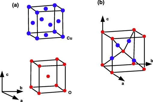
Crystallographic structure of Molecule
. (a) Structural characteristics of Cu and O atoms in the
lattice. The
lattice is formed by interpenetrating the Cu and O lattices with each other. (b) Unit cell of
. Copper atoms are shown as small blue spheres, and oxygen atoms are shown as large red spheres. In the
lattice, each Cu atom is coordinated with two O atoms, and each O atom is coordinated with four Cu atoms.
![Crystallographic structure of Cu 2 O [ 3 , 2 , 3 ] .](/content/184/2020/13/8/img/10.1016_j.arabjc.2020.05.021-fig2.png)
Crystallographic structure of
.
To compute our result we make the partitions of the vertices and edge. More preciously the vertex partition of
based on degrees of each vertex is depicted in Table 1. Also the edge partition of
based on degrees of end vertices of each edge are depicted in Table 2.
Frequency
Set of Vertices
1
2
4
Frequency
Set of Edges
6.1 Results for crystallographic structure of
In this section we computes the entropies of the crystallographic Structure of molecule .
-
The Redefined First Zagreb Entropy of
Now using Eq. (2), and Table 2, we computed the Redefined first Zagreb entropy in the following way:
It is easy to see that the Redefined first Zagreb index by using Table 2 is Since has three types of edges, So Eq. (2), with Table 2 can take the form: Now using the value of the Redefined first Zagreb index in above equation, we obtained the exact value of Redefined first Zagreb entropy in following expression.
-
The Redefined Second Zagreb Entropy of
Now using Eq. (3), and Table 2, we computed the Redefined second Zagreb entropy in the following way:
It is easy to see that the Redefined second Zagreb index by using Table 2 is Since has three types of edges, So Eq. (3), with Table 2 can take the form: Now using the value of the Redefined second Zagreb index in above equation, we obtained the exact value of Redefined second Zagreb entropy in following expression.
-
The Redefined Third Zagreb Entropy of
Now using Eq. (4), and Table 2, we computed the Redefined third Zagreb entropy in the following way:
It is easy to see that the Redefined third Zagreb index by using Table 2 is Since has three types of edges, So Eq. (4), with Table 2 can take the form: Now using the value of the Redefined third Zagreb index in above equation, we obtained the exact value of Redefined third Zagreb entropy in following expression.
-
The Fourth Atom Bond Connectivity Entropy of
The Table 3 shows the edge partition of the chemical graph
based on the degree sum of end vertices of each edge.
Frequency
Set of Edges
Now using Eq. (5), and Table 3, we computed the fourth atom bond connectivity entropy in the following way:
It is easy to see that the fourth atom bond connectivity index by using Table 3 is
-
The Fifth Geometric Arithmetic Entropy of
Now using Eq. (6), and Table 3, we computed the fifth geometric arithmetic entropy in the following way:
It is easy to see that the fifth geometric arithmetic index by using Table 3 is:
-
The Sanskruti Entropy of
Now using Eq. (7), and Table 3, we computed the Sanskruti entropy in the following way:
It is easy to see that the Sanskruti index by using Table 3 is: Since has five types of edges, So Eq. (7), with Table 3 can take the form: Now using the value of the Sanskruti index, we obtained the exact value of Sanskruti entropy in following expression.
7 Crystallographic Structure of
Titanium Difluoride is a water insoluble Titanium source for use in oxygen-sensitive applications, such as metal production. Fluoride compounds have diverse applications in current technologies and science, from oil refining and etching to synthetic organic chemistry and the manufacture of pharmaceuticals. The chemical graph of crystal structure of titanium difluoride
is described in Fig. 3, for more details see (Cotton et al., 1999). Let
be the chemical graph of
with
unit cells in the plane and t layers. We construct this graph first by taking
unites in the
-plane and then storing it up in t layers. The number of vertices and edges of
are
and
, respectively.![Crystal Structure Titanium Difluoride TiF 2 [ m , n , t ] , (a) represents unit cell of TiF 2 [ m , n , t ] with Ti atoms in red and F atoms in green (b) crystal structure of TiF 2 [ 4 , 1 , 2 ] .](/content/184/2020/13/8/img/10.1016_j.arabjc.2020.05.021-fig3.png)
Crystal Structure Titanium Difluoride
, (a) represents unit cell of
with Ti atoms in red and F atoms in green (b) crystal structure of
.
To compute our result we make the partitions of the vertices and edge. More preciously the vertex partition of
based on degrees of each vertex is depicted in Table 4. Also the edge partition of
based on degrees of end vertices of each edge are depicted in Table 5.
Frequency
Set of Vertices
1
8
2
4
8
Frequency
Set of Edges
8
7.1 Results for Crystallographic Structure of
In this section we computes the entropies of the Crystal Structure of Titanium Difluoride .
-
The Redefined First Zagreb Entropy of
Now using Eq. (2), and Table 5, we computed the Redefined first Zagreb entropy in the following way:
It is easy to see that the Redefined first Zagreb index by using Table 5 is Since has three types of edges, So Eq. (2), with Table 5 can take the form: Now using the value of the Redefined first Zagreb index in above equation, we obtained the exact value of Redefined first Zagreb entropy in following expression.
-
The Redefined Second Zagreb Entropy of
Now using Eq. (3), and Table 2, we computed the Redefined second Zagreb entropy in the following way:
It is easy to see that the Redefined second Zagreb index by using Table 2 is Since has three types of edges, So Eq. (3), with Table 2 can take the form: Now using the value of the Redefined second Zagreb index in above equation, we obtained the exact value of Redefined second Zagreb entropy in following expression.
-
The Redefined Third Zagreb Entropy of
Now using Eq. (4), and Table 5, we computed the Redefined third Zagreb entropy in the following way:
It is easy to see that the Redefined third Zagreb index by using Table 5 is Since has three types of edges, So Eq. (4), with Table 5 can take the form: Now using the value of the Redefined third Zagreb index in above equation, we obtained the exact value of Redefined third Zagreb entropy in following expression.
-
The Fourth Atom Bond Connectivity Entropy of
The Table 6 shows the edge partition of the chemical graph
based on the degree sum of end vertices of each edge.
Frequency
Set of edges
8
16
Now using Eq. (5), and Table 6, we computed the fourth atom bond connectivity entropy in the following way:
It is easy to see that the fourth atom bond connectivity index by using Table 6 is:
-
The Fifth Geometric Arithmetic Entropy of
Now using Eq. (6), and Table 6, we computed the fifth geometric arithmetic entropy in the following way:
It is easy to see that the fifth geometric arithmetic index by using Table 6 is: Since has six types of edges, So Eq. (6), with Table 6 can take the form: Now using the value of the fifth geometric arithmetic index from Eq. (9), we obtained the exact value of fifth geometric arithmetic entropy in following expression.
-
The Sanskruti Entropy of
Now using Eq. (7), and Table 6, we computed the Sanskruti entropy in the following way:
It is easy to see that the Sanskruti index by using Table 6 is: Since has six types of edges, So Eq. (7), with Table 6 can take the form: Now using the value of the Sanskruti index, we obtained the exact value of Sanskruti entropy in following expression.
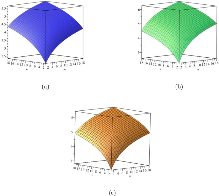
8 Comparisons and discussion for
Since the degree based entropy has lot of application in different branches of science, namely pharmaceutical, chemistry, biological drugs and computer science. So the numerical and graphical representation of these calculated results are helpful to scientist. So in this section, we have computed numerically all degree based entropies for different values of
for
. In addition, we construct Tables 7, 8 for small values of
for degree based entropy to numerical comparison for the structure of
. Now, from Tables 7, 8, we can easily see that all the values of entropy are in increasing order as the values of
are increases. The graphical representations of computed results are depicted in Fig. 4 and Fig. 5 for certain values of
.
(a) The Redefined first Zagreb entropy, (b) The Redefined second Zagreb entropy, (c) The Redefined third Zagreb entropy.
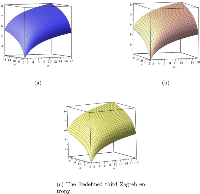
(a) The
entropy, (b) The
entropy, (c) The Sanskruti entropy.
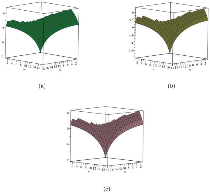
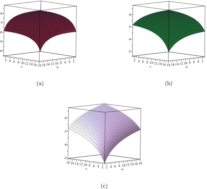
9 Comparisons and discussion for
Since the degree based entropy has lot of application in different branches of science, namely pharmaceutical, chemistry, biological drugs and computer science. So the numerical and graphical representation of these calculated results are helpful to scientist. So in this section, we have computed numerically all degree based entropies for different values of
for
. In addition, we construct Tables 9, 10 for small values of
for degree based entropy to numerical comparison for the structure of
. Now, from Tables 9, 10, we can easily see that all the values of entropy are in increasing order as the values of
are increases. The graphical representations of computed results are depicted in Fig. 6 and Fig. 7 for certain values of
.
(a) The Redefined first Zagreb entropy, (b) The Redefined second Zagreb entropy, (c) The Redefined third Zagreb entropy.
(a) The
entropy, (b) The
entropy, (c) The Sanskruti entropy.
10 Conclusion
In this paper, based on Shannon,s entropy and Chen et.al entropy definitions, we study the graph entropies related to a new information function. We introduces a relation between the degree based topological indices with degree based entropies. We computed the degree based entropies for crystallographic Structure of Copper Oxide and Titanium Difluoride . We also computed the numerical values of these entropies in Tables and give the comparison between the degree based topological indices and degree based entropies, which leads us to know the Physico-chemical properties of these crystallographic Structure of Copper Oxide and Titanium Difluoride .
In future, we want to extended this idea other chemical structures which explore the new direction of researcher in this field.
Acknowledgment
The authors would like to thanks the two anonymous reviewers for their very constructive comments that helped us to enhance the quality of this manuscript.
References
- Complexity in Chemistry, Introduction and Fundamentals. Boca Raton, FL, USA: Taylor and Francis; 2003.
- Degree-based entropies of networks revisited. Appl. Math. Comput.. 2015;261:141-147.
- [Google Scholar]
- Advanced Inorganic Chemistry. John Wiley and Sons; 1999.
- Information processing in complex networks: Graph entropy and information functionals. Appl. Math. Comput.. 2008;201:82-94.
- [Google Scholar]
- The discrimination power of molecular identification numbers revisited. MATCH Commun. Math. Comput. Chem.. 2013;69:785-794.
- [Google Scholar]
- Uniquely discriminating molecular structures using novel eigenvalue-based descriptors. MATCH Commun. Math. Comput. Chem.. 2012;67:147-172.
- [Google Scholar]
- Generalized walks-based centrality measures for complex biological networks. J. Theor. Biol.. 2010;263:556-565.
- [Google Scholar]
- Statistical-mechanical approach to subgraph centrality in complex networks. Chem. Phys. Lett.. 2007;439:247-251.
- [Google Scholar]
- Topological characterization of carbon graphite and crystal cubic carbon structures. Molecules. 2017;22:1496-1507.
- [Google Scholar]
- Study of biological networks using graph theory. Saudi J. Biol. Sci.. 2018;25:1212-1219.
- [Google Scholar]
- Computing ABC4 index of nanostar dendrimers. Optoelectron. Adv. Mater.-Rapid Commun.. 2010;4:1419-1422.
- [Google Scholar]
- Computing fifth geometric-arithmetic index for nanostar dendrimers. J. Math. Nanosci.. 2011;1:33-42.
- [Google Scholar]
- Computing Sanskruti index of certain nanostructures. J. Appl. Math. Comput. 2016
- [CrossRef] [Google Scholar]
- On topological properties of symmetric chemical structures. Symmetry. 2018;10(173):1-21.
- [Google Scholar]
- Some order-disorder considerations in living systems. Bull. Math. Biophys.. 1953;17:81-86.
- [Google Scholar]
- Ranjini, P.S., Lokesha, V., Usha, A., 2013. Relation between phenylene and hexagonal squeez using harmonic index. Int. J. Graph Theory 1, 116–121.
- On zagreb indices, zagreb polynomials of some nanostar dendrimers. Appl. Math. Comput.. 2016;280:132-139.
- [Google Scholar]
- Computing topological indicesof certain networks. J. Optoelectron. Adv. Mater.. 2016;18(9–10):884-892.
- [Google Scholar]
- Information theory of complex networks: on evolution and architectural constraints. Complex Netw. Lect. Notes Phys.. 2004;650:189-207.
- [Google Scholar]
- Network structure entropy and its application to scale-free networks. Syst. Eng.-Theory Pract.. 2004;6:1-3.
- [Google Scholar]
- A note on the information content of graphs. Bull. Math. Biol.. 1956;18(2):129-135.
- [Google Scholar]
- Quantitative methods for ecological network analysis. Comput. Biol. Chem.. 2004;28:321-339.
- [Google Scholar]
- Quantitative structure-property relationship (QSPR) modeling of drug-loaded polymeric micelles via genetic function approximation. PLoS ONE. 2015;10(3):119-129.
- [Google Scholar]
- Nearly monodisperse Cu2O and CuO nanospheres: preparation and applications for sensitive gas sensors. Chem. Mater.. 2006;18:867-871.
- [Google Scholar]


