

Translate this page into:
On analysis of heat of formation and entropy measures for indium phosphide
-
Received: ,
Accepted: ,
This article was originally published by Elsevier and was migrated to Scientific Scholar after the change of Publisher.
Abstract
A chemical graph represents a chemical or molecular compound in the form of a graph. The vertex set of the chemical graph contains the atoms or molecules of the compound while the edge set comprises of the bonding between the molecules or atoms. In this paper, we compute various connectivity indices based on degrees of vertices of chemical graph of Indium Phosphide (InP) including general Randić, hyper Zagreb and redefined Zagreb indices etc. Afterwards, we calculate the physical measures such as entropy and heat of formation of InP. We fit curves between different indices and the thermodynamical properties namely heat of formation and entropy by using MATLAB through different methods based on linearity and non-linearity. The performance of the method is tested using root mean square error, the sum of squared errors or . Furthermore, we give graphical representations of these indices. These mathematical frameworks might provide a way to study the thermodynamical properties of the chemical structure of InP at different conditions which will assist to comprehend the relationship between system dimension and these measures.
Keywords
Network
Connectivity index
Indium phosphide
Entropy
Heat of formation
Statistical tests

1 Introduction
The term used to illustrate a molecular/chemical compound in the form of a graph is known as molecular/chemical graph (Baig et al., 2017; Gao et al., 2018). Molecules are shown as vertices while their bondings or interactions are shown by edges in a molecular graph. Usually, molecule graphs are simple graphs and the measure of topological index is invariant under graph isomorphisms. Mostly, the degree or distance measure is used to capture the topology of a graphical structure so the most common indices are based on either degree or distance between the vertices. Indices comprising of degree measurements perform a vigorous part in molecular graph theory. Two isomorphic graphs have same connectivity index and the cardinalities of vertex and edge sets of a graph are considered as the topological/connectivity indices as well. A connectivity index explains some helpful details about structure and analysis of molecular graph. An application of graph theory in the field of chemistry is to study the molecular structures of chemical compounds. Graph theory tools are implemented to classify fundamental features entailed in structure–property activity interactions of molecules. Many chemical compounds have been analyzed through topological indices in the past few decades. Topological/graphical index is a numeric measure related to chemical compositions asserting the association of chemical structures through numerous physicochemical properties or chemical reactivity (Baig et al., 2017).
A. Balaban, A. Graovac, I. Gutman, H. Hosoya, M. Randić, and N. Trinajsti (Randić, 2004) are originators of the field of chemical graph theory. It was acknowledged in 1988 that a lot of researchers had worked in this field and published roughly 500 publications per year see details (Ahmad et al., 2019; Ahmad et al., 2020; Aslam et al., 2019; Li et al., 2021). Chemical graph theory, a 2-volume comprehensive treatise by Trinajsti, that conveyed the research up to the mid of 1980’s, is one of many monographs in the discipline (Das and Gutman, 2004). Zhang et al. (2018), Zhang et al. (2019), Zhang et al. (2020) discuss the topological indices of generalized bridge molecular graphs, Carbon Nanotubes and product of chemical graphs.
Chemical compounds are represented by graphs in chemical graph theory, and mathematical tools are employed to address chemistry issues. A topological/connectivity descriptor is a numerical measure which describes the topology of a graph (Gutman et al., 2015). These are sensitive to symmetry, heteroatom content, magnitude, form, connecting style, and the degree of intricacy of atomic regions, among other structural features of molecules (Hayat and Imran, 2015; Manzoor et al., 2021). Connectivity descriptors have gained considerable popularity recently, due to their simple nature. Chemical graph theory relies considerably on these graph descriptors. As a consequence, a topological index may be quantitatively characterizes a chemical network that is topologically invariant to labelling as well as distinguish between isomers (Gao et al., 2017; Shannon, 1948). Zhang et al. (2018, 2021) provided the physical analysis of heat for formation and entropy of Ceria Oxide.
In theoretical chemistry and nanotechnology, there are several graphs associated numerical descriptors that are significant. Degree-based, distance-based, and counting-related graph descriptors are among the most common types (Furtula et al., 2010). The degree-based graph descriptors have a prominent place among these descriptors and may be used to characterises chemical substances and forecast their specific physio-chemical characteristics (Amić et al., 1998; Bollobs and Erdos, 1998; Došlić, 2008; Furtula and Gutman, 2015; Gutman and Trinajsti, 1972; Khalid et al., 2022; Siddiqui et al., 2016).
Researchers are working in the field of connectivity/topological indices in different ways; some are just developing them as graph descriptors (Furtula et al., 2014; Gao et al., 2017; Shao et al., 2018; Siddiqui et al., 2016) while some are relating them with certain molecules to analyze their chemical properties (Gao et al., 2018).
To construct a thermodynamical structure we need to measure some physical quantities, entropy (Ent) and heat of formation (HoF) are two of them.
Ent measure tells us how much heat energy we need to produce more in order to perform some valued work. Since this measure is describing the lack of energy due to which performing valuable work is not possible so it is also termed as measure of disorder (Dehmer and Mowshowitz, 2011; Estrada et al., 2014). An isolated system has the highest Ent according to the second law of thermodynamics. Non-isolated systems can lose Ent if they enhance the Ent of their surroundings by at least the same amount. Because Ent is a state function, every process that moves a system from one state to another, whether reversible or irreversible, will change its Ent.
During per unit formation, the heat absorbed or retained is referred as HoF provided all the elements persist in normal state. Kilojoules per mole (kJ/mol) is the unit for the measure of HoF. The term enthalpy is also used for HoF.
Defining a system in the form of a mathematical framework provides us an efficient approach to analyze the dynamics of the system. Experimental work is mostly expensive and very time consuming so transforming the system into a set of mathematical form makes this study very coherent. Many softwares like MATLAB or Python are easily available which provide a very friendly environment to construct mathematical models and study them. As we may fit many mathematical models to the same set of data so it is difficult to decide which one is best suitable for us. There are several statistical tests which might help us to decide which mathematical model or framework is a best fit for our data but we will just consider RMSE, and SSE.
In (Chu et al., 2021; Siddiqui et al., 2021; Ma et al., 2021; Zhang et al., 2022; Zhao et al., 2020), authors estimated the mathematical frameworks to detect relationships between physical measures including Ent and HoF and degree based topological indices of ceria oxide, graphite carbon nitride and terbium IV. In (Khalid et al., 2022), Khalid et al. found a network of indices to capture the subnetwork consisting of highly most connected indices of the drug Astragaloside IV. Gao et al. (2018) introduced the concept of HoF and Ent measures for Copper (I) Oxide and Copper (II) Oxide based on the topological indices. Nadeem et al. (2019) extended this idea for 2-Dimensional Silicon Carbons. Manzoor et al. (2020) provided detailed information about this idea and applied for new structures namely carbon nanosheets.
2 Crystal structure of indium phosphide
The binary semiconductor indium phosphide (InP) is made up of the elements indium besides phosphorus. Its structure is similar to other crystal structure of majority of group
semiconductors which have face-centered cubic configuration (Vurgaftman et al., 2001) as shown in Fig. 1. Indium phosphide is either synthesized by reacting red phosphorous powder with indium iodide at 400 °C or by combining refined high temperatures and pressures elements, or by thermal disintegration of a combination of trialkyl indium compounds and phosphine as shown in Fig. 2 (Zafar and Iqbal, 2016). Electrochemical etching of indium phosphide nano-crystalline surface was viewed by scanning electron microscope.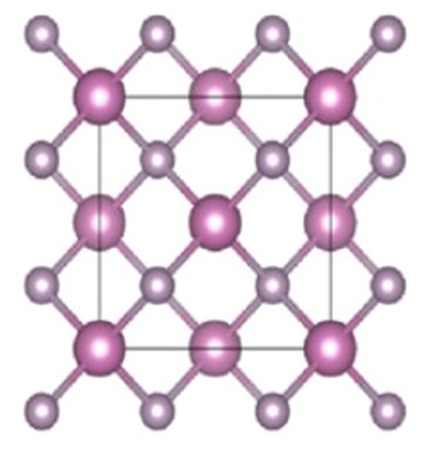
Crystal structure of indium phosphide (InP).
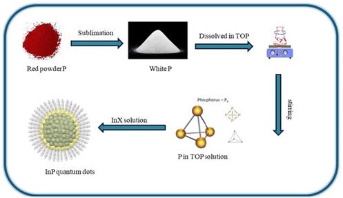
Scheme for the synthesis of InP QDs.
Because of their large direct current, Group IIIA phosphide nano-crystalline semiconductors are of great interest among the significant inorganic materials. They have fundamental physical properties and band differences (Zafar and Iqbal, 2016). Its unique properties like low dielectric, low density and high thermal conductivity in comparison to the common semiconductors like Si, Ga and As (Ozkendir, 2020; Souza, 1996) makes it more useful in high power and high-frequency electronics. Conventionally Cd and Pb halides are being used in display technology but their toxicity limits their use in color technology. Because of their reduced toxicity and emission tunability range from visible to near-infrared, indium phosphide quantum dots (QDs) are an appealing option. Semiconductor nanocrystals, also known as quantum dots, are nanometer-sized fluorescent materials that can have their optical properties fine-tuned by changing the core size or expanding a shell around the core (Mushonga, 2012). Because of its superior electron velocity to the more popular semiconductors Si, Ga and As, it is used in high-power and high-frequency electronics. InP is also used as a medium for epitaxial materials (Kerkouri et al., 2011). The QDs of indium phosphide are now being used in heavy metals detection as an alternative to cadmium-based materials (Bouarissa, 2011).
Lasers and LEDs based on InP can emit light with a wavelength range of to . This light is used in all parts of the digitalized world for fibre-based telecom and datacom applications. Light can also be utilized for sensing purposes. On the one side, there are spectroscopic applications in which a certain wavelength is used to interfere with matter, such as in the detection of highly diluted gases. In the automobile industry, optoelectronic terahertz is used for ultra-sensitive spectroscopic analysers, polymer thickness tests, and multilayer coating identification. Relevant InP lasers have a tremendous advantage in terms of eye protection. The radiation is absorbed by the human eye vitreous body which has little effect on the retina.
3 Methods
This section is devoted to discuss the methods used to establish the relationships between thermodynamics properties of InP and the graphical properties of its corresponding chemical graph. Firstly, various topological indices are found based on the degrees of the vertices including Randić index, redefined Zagreb and hyper-Zagreb indices, general forms of few of them are listed below. Let be a graph and denote the degree of a vertex u.
General Randić index introduced in (Randić, 1975; Soleimani et al., 2015) is as follows: Shirdel et al. introduced hyper-Zagreb index in (Ghorbani and Azimi, 2012) as given below. Afterwards, HoF and Ent of InP are obtained for different formula unit cells of InP. For one formula unit standard molar HoF and Ent are calculated by dividing them by Avogadro’s number. The HoF and Ent of a cell are calculated by multiplying the obtained values by the number of formula units within the cell. Topological indices vs different formula unit cells are shown by graphical illustrations. Non-linear graphical models are fitted by considering topological indices as input variables and enthalpy and entropy as output variables. Finally, various curves are fitted using curve fitting app in MATLAB. Several built in methods are available in the curve fitting app, we implement most of them on our data. The statistical tests are the best tools to select the best mathematical model for the given data. Let be our data set and n be the number of observations. Suppose that be the set of fitted values corresponding to Y. The standard deviation is an important feature and shows how much deviation we have in our values from mean and keeping this value in consideration provides a more accurate fit to our data. To calculate an error using standard deviation we use root mean squared error (RMSE), which is defined as following: RMSE shows standard deviation of the residuals (i.e. difference between the model predictions and the true values). This test provides an estimate of how large the residuals are being dispersed. It can be easily interpreted in the form of mean squared error (MSE) as RMSE is just the square root of MSE.
Another statistical test is sum of squared error defined as following: -test is used to analyze how observed values are scattered from our fitted curve. The value of approaching to 1 shows good fit while approaching to zero shows poor estimation. is the ratio between calculated and actual variance. Suppose that S is the variance of fit and is actual variance then the formula of is given below: There are few other statistical tests in the literature as well but the curve fitting app in MATLAB selects the model based on and only so we will consider these three tests.
4 Degree based indices for indium phosphide
The number of vertices and edges of InP[s, t] are 10st + 3s + 3t + 2 and 16st, respectively for unit cells. Furthermore, Table 1 gives details about the edge partition whereas the comparisons of the indices for InP[s, t] are given in Table 2 and Table 3.
Let with . Then the Randić indices for are as follows:
For For For For □
| Frequency(Total Number of Edges) | Set of Edges | |
|---|---|---|
| 112 | ||||
| 560 | 8 | |||
| 1328 | ||||
| 2416 | 25 | |||
| 3824 | ||||
| 5552 | 50 | |||
| 7600 |
| 14 | 656 | 532 | ||
| 47 | 3824 | 2476 | ||
| 94 | 192 | 9424 | 5732 | |
| 155 | 17456 | 10300 | ||
| 230 | 27920 | 16180 | ||
| 319 | 40816 | 23372 | ||
| 422 | 56144 | 31876 |
The numerical representation of above computed results are depicted in Table 2.
The hyper Zagreb index for the graph of with is corresponding to
Let denote InP crystallographic structure. The following is the hyper Zagreb index result: □
The redefined Zagreb indices for the graph of with is corresponding to
Let denote InP crystallographic structure. The redefined Zagreb indices are as follows: □
The numerical representation of above computed results are depicted in Table 3. Graphical behaviours of Randić indices and redefined Zagreb indices for different formula unit cells of InP are illustrated in Fig. 3, Fig. 4 and Fig. 5 respectively.![Comparison of Randić indices for α = 1 , - 1 , 1 2 , - 1 2 for InP[s, t].](/content/184/2022/15/11/img/10.1016_j.arabjc.2022.104218-fig3.png)
Comparison of Randić indices for
=
for InP[s, t].
![Comparison of ReZG 1 ( G ) , ReZG 2 ( G ) , ReZG 3 ( G ) indices for InP[s, t].](/content/184/2022/15/11/img/10.1016_j.arabjc.2022.104218-fig4.png)
Comparison of
indices for InP[s, t].
![Graphical representation of HM ( G ) for unit cells of InP[s, t].](/content/184/2022/15/11/img/10.1016_j.arabjc.2022.104218-fig5.png)
Graphical representation of
for unit cells of InP[s, t].
5 Heat of formation and entropy of indium phosphide
The standard molar HoF of InP is
, whereas the standard molar Ent of indium phosphide is
. The enthalpy of indium phosphide is inversely proportional to its crystal size, and increases as the number of unit cells increases. If the number of cells grows larger, the Ent value decreases. The downward trend is the exact opposite of HoF. These numerical findings are represented in Table 4.
Formula units
HoF
kJ
Ent
kJ
4
16
36
64
100
144
196
6 Results and discussion
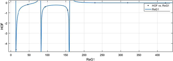
In this section, results of this article are presented which include the estimation of the mathematical frameworks describing the relationships between each index found in Section 4 and each physical measure found in Section 5. Few of the results are presented here while remaining results are provided in the supplementary material. A mathematical model between the index
and HoF is estimated in (1).
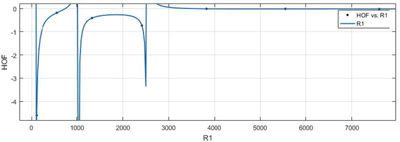
(x-axis) vs HoF (y-axis).
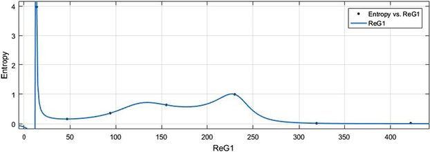
In the case of entropy, the values of
are again normalized by the same mean
and std
. The estimated model is presented in (2) where
,
,
with
.
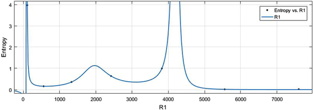
(x-axis) vs Ent (y-axis).
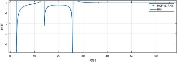
To estimate the models of index
vs HoF and
vs Ent, the values of
are normalized by mean
and std
in both cases. The estimated models are presented in (3) and (4) with parametric values
for (3) and
for (4).
vs HoF.
vs Ent.
vs HoF.
vs HoF.
vs HoF.
HM vs HoF.
vs HoF.
vs HoF.
vs Ent.
vs Ent.
vs Ent.
HM vs Ent.
vs Ent.
vs Ent.
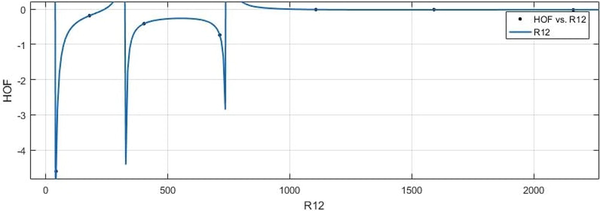
The mathematical connections between indices and HoF and Ent are provided in the following along with the parametric values and confidence interval (CI), and their goodness of fit.
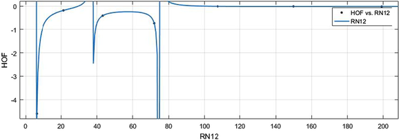
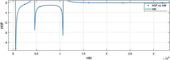
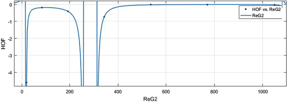
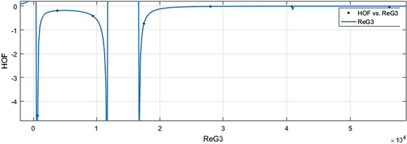
6.1 HoF vs Indices
The general models for all the indices are given in (5)–(10) while graphical representation for all the indices vs HoF are shown in Figs. 10–15.
-
General model between and HoF
Coefficients with CI:
.
Goodness of fit:
.
-
General model between and HoF
Coefficients with CI:
.
Goodness of fit:
.
-
General model between and HoF
Coefficients with CI:
.
Goodness of fit:
.
-
General model between HM and HoF
Coefficients with CI:
.
Goodness of fit:
.
-
General model between and HoF
Coefficients with CI:
.
Goodness of fit:
.
-
General model between and HoF
Coefficients with CI:
.
Goodness of fit:
.
6.2 Ent vs Indices
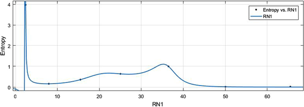
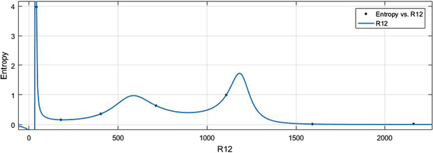
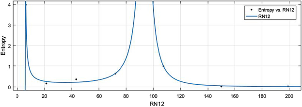
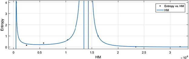
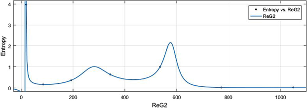
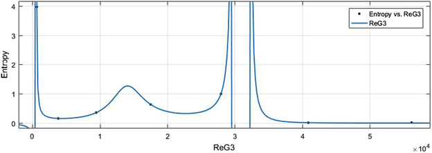
The general models between Ent and different indices are given in (11)–(16) while their graphical representation for all indices vs Ent are shown in Figs. 16–21.
-
General model between and Ent
Coefficients with CI:
.
Goodness of fit:
.
-
General model between and Ent
Coefficients with CI:
.
Goodness of fit:
.
-
General model between and Ent
Coefficients with CI:
.
Goodness of fit:
.
-
General model between HM and Ent
Coefficients with CI:
.
Goodness of fit:
.
-
General model between and Ent
Coefficients with CI:
.
Goodness of fit:
.
-
General model between and Ent
Coefficients with CI:
.
Goodness of fit:
.
7 Conclusion
In this paper, we investigated the relationships between the underlying graphical properties and the thermodynamical properties of indium phosphide. At first the topological degree based indices were calculated which were lately integrated with thermodynamical properties of indium phosphide InP[s, t] to form mathematical formulations. Such links had been established by fitting curve between each index and each thermodynamical property. Ent and HoF are two types of thermodynamical properties which were indulged in this study. Rational fitting method was applied using MATLAB software as this method was providing the least root mean squared error or sum of squared error among all built in methods. The graphical behaviours of such established connections were also shown which provided the values of the indices where HoF and Ent measure changed their behaviours. Such a multidisciplinary approach would provide a comprehensive insight to understand the structural properties of indium phosphide InP[s, t] in more detail and depth.
Funding
This research is supported by the UAEU-AUA (Asian Universities Alliance) grants of United Arab Emirates University (UAEU) via Grant No. G00003461.
Declaration of Competing Interest
The authors declare that they have no known competing financial interests or personal relationships that could have appeared to influence the work reported in this paper.
References
- Computing the degree based topological indices of line graph of benzene ring embedded in P-type-surface in 2D network. J. Informat. Optim. Sci.. 2019;40(7):1511-1528.
- [Google Scholar]
- Eccentric connectivity indices of titania nanotubes TiO2 [m; n] Eurasian Chem. Commun.. 2020;2(6):712-721.
- [Google Scholar]
- The vertex-connectivity index revisited. J. Chem. Informat. Comput. Sci.. 1998;38(5):819-822.
- [Google Scholar]
- Computing certain topological indices of the line graphs of subdivision graphs of some rooted product graphs. Mathematics. 2019;7(5):393-403.
- [Google Scholar]
- Molecular description of carbon graphite and crystal cubic carbon structures. Can. J. Chem.. 2017;95(6):674-686.
- [Google Scholar]
- Phonons and related crystal properties in indium phosphide under pressure. Phys. B: Condensed Matter. 2011;406(13):2583-2587.
- [Google Scholar]
- On Zagreb Type Molecular Descriptors of Ceria Oxide and Their Applications. J. Cluster Sci. 2021
- [Google Scholar]
- Some properties of the second Zagreb index. MATCH Commun. Math. Comput. Chem. 2004;52(1):33-41.
- [Google Scholar]
- Vertex-weighted Wiener polynomials for composite graphs. Ars Mathematica Contemporanea. 2008;1(1):66-80.
- [Google Scholar]
- Topological characterization of carbon graphite and crystal cubic carbon structures. Molecules. 2017;22(9):14-26.
- [Google Scholar]
- Topological characterization of carbon graphite and crystal cubic carbon structures. Molecules. 2017;22(9):1496-1515.
- [Google Scholar]
- Molecular description of copper (I) oxide and copper (II) oxide. Quim. Nova. 2018;41(8):874-879.
- [Google Scholar]
- Graph theory and molecular orbitals. Total electron energy of alternant hydrocarbons. Chem. Phys. Lett.. 1972;17(4):535-538.
- [Google Scholar]
- On Zagreb indices and coindices. MATCH Commun. Math. Comput. Chem. 2015;74(1):5-16.
- [Google Scholar]
- Computation of certain topological indices of nanotubes covered by . J. Comput. Theor. Nanosci.. 2015;12(4):533-541.
- [Google Scholar]
- FTIR, Raman, EPR and optical absorption spectral studies on V2O5-doped cadmium phosphate glasses. Physica B. 2011;406(17):3142-3148.
- [Google Scholar]
- On topological analysis of astragaloside IV drug using network construction and module detection. Eur. Phys. J. Plus. 2022;137:214.
- [Google Scholar]
- Valency-based topological properties of linear hexagonal chain and hammer-like benzenoid. Complexity. 2021;2021:1-16.
- [Google Scholar]
- Yanli Ma, Muhammad Kamran Siddiqui, Sana Javed, Lubna Sherin, 2021. On Analysis of Topological Indices for Graphitic Carbon Nitride via Enthalpy and Entropy Measurements, Polycyclic Aromatic Compounds, Polycyclic Aromatic Compounds.
- On topological aspects of degree based entropy for two carbon nanosheets. Main Group Met. Chem... 2020;43:205-218.
- [Google Scholar]
- On physical analysis of degree-based entropy measures for metal–organic superlattices. Eur. Phys. J. Plus. 2021;136(3):1-22.
- [Google Scholar]
- Indium phosphide-based semiconductor nanocrystals and their applications. J. Nanomater. 2012:20-35.
- [Google Scholar]
- Topological Descriptor of 2-Dimensional Silicon Carbons and Their Applications. Open Chem.. 2019;17:1473-1482.
- [Google Scholar]
- Electronic structure study of Sn-substituted InP semiconductor. Adv. J. Sci. Eng.. 2020;1(1):7-11.
- [Google Scholar]
- Nenad Trinajsti–pioneer of chemical graph theory. Croatica Chem. Acta. 2004;77(1–2):1-15.
- [Google Scholar]
- Computing zagreb indices and zagreb polynomials for symmetrical nanotubes. Symmetry. 2018;10(7):244-260.
- [Google Scholar]
- On Zagreb indices, Zagreb polynomials of some nanostar dendrimers. Appl. Mathe. Comput.. 2016;280:132-139.
- [Google Scholar]
- Computing topological indices of certain networks. J. Optoelectron. Adv. Mater.. 2016;18(16):884-892.
- [Google Scholar]
- Siddiqui, M.K., Javed, S., Sherin, L., Khalid, S., Muhammad Mathar Bashir, Amir Hassan, Mlamuli Dhlamini, 2021. On Analysis of Topological Properties for Terbium IV Oxide via Enthalpy and Entropy Measurements, J. Chem. 2021, 16 pages, Article ID 5351776.
- Computation of the different topological indices of nanostructures. J. National Sci. Found. Sri Lanka. 2015;43(2)
- [Google Scholar]
- Electron and irradiation effects in InP assessed by photoluminescence. J. Appl. Phys.. 1996;79(7):3482-3486.
- [Google Scholar]
- Band parameters for III–V compound semiconductors and their alloys. J. Appl. Phys.. 2001;89(11):58-75.
- [Google Scholar]
- Indium phosphide nanowires and their applications in optoelectronic devices. Proc. Roy. Soc. A: Mathe. Phys. Eng. Sci.. 2016;472(2187):201-214.
- [Google Scholar]
- Edge-version atom-bond connectivity and geometric arithmetic indices of generalized bridge molecular graphs. Symmetry. 2018;10(12):751-786.
- [Google Scholar]
- The cartesian product and join graphs on edge-version atom-bond connectivity and geometric arithmetic indices. Molecules. 2018;23(7):1-17.
- [Google Scholar]
- On degree based topological properties of two carbon nanotubes. Polycyclic Aromat. Compd.. 2020;10:22-35.
- [Google Scholar]
- Study of Hardness of Superhard Crystals by Topological Indices. J. Chem.. 2021;10:7-20.
- [Google Scholar]
- Physical Analysis of Heat for Formation and Entropy of Ceria Oxide Using Topological Indices. Comb. Chem. High Throughput Screen.. 2022;25(3):441-450.
- [Google Scholar]
- Molecular topological indices-based analysis of thermodynamic properties of graphitic carbon nitride. Eur. Phys. J. Plus. 2020;135(12):1-19.
- [Google Scholar]


