

Translate this page into:
A CFD examination of free convective flow of a non-Newtonian viscoplastic fluid using ANSYS Fluent
⁎Corresponding author. m_r_eid@yahoo.com (Mohamed R. Eid)
-
Received: ,
Accepted: ,
This article was originally published by Elsevier and was migrated to Scientific Scholar after the change of Publisher.
Peer review under responsibility of King Saud University.
Abstract
In this work, a laminar steady-state investigation of free convection in a square cavity with differential heated side walls is examined. The cavity is immersed with a viscoplastic liquid the Bingham prototype. The horizontal walls are assumed as adiabatic and the vertical wall has two spatial differing sinusoidal temperature profiles with diverse phases and amplitudes. The hydro-thermal features are systematically analyzed via a broad choice of Rayleigh numbers (103-106), Bingham numbers , Prandtl numbers (0.1, 1, 10), amplitude ratio (0–––1), phase difference (0-π) and flow index (0.3–2). The governing equations are treated computationally utilizing a commercial computational simulation code CFD: FLUENT. It has been observed that average Nusselt numbers grow with growing Rayleigh numbers and drop with increasing Bingham quantity , since heat transition occurs primarily due to thermic conductivity. In general, a higher Rayleigh number promotes convection and increases heat transfer efficiency, leading to a higher Nusselt number, whereas a higher Bingham number, indicating a higher degree of viscous or yield-stress behavior, may inhibit convection and decrease heat transfer efficiency, which ended in a lower Nusselt number. These connections frequently appear in heat transport and fluid dynamics simulations. The rise in the phase difference suggests an upsurge in heat transference, as the impact of the phase shift on the Nusselt is perpetually enhanced due to the amount of Rayleigh boosts for all phase differences. Heat transition rate for is boosted because of the values. Moreover, when the amplitude ratio goes up, so does heat transfer. The gap between average Nusselt and Rayleigh amounts rose as the Rayleigh rose. The thermal flow rate is bigger in than in the other cases. The rise in phase difference suggests a rise in heat transference, as this effect of phase shift on Nusselt continues to be enhanced due to the amount of Rayleigh boosts for all phase differences. Heat transition rate is enhanced for based on the values. Plus, when the amplitude ratio grows, so does heat transmission. The rate of heat transport for is larger than in the other cases.
Keywords
Bingham fluid
Free convection flow
CFD
ANSYS Fluent
Square heated cavity

Nomenclature
-
correlation parameters
-
aspect ratio
-
dimensionless temperature difference
-
Bingham number
-
heat capacity
-
Grashof number
-
Gravity
-
Height
-
consistency
-
domain length
-
Pressure
-
Prandtl number
-
Rayleigh number
-
Nusselt number
-
temperature
-
hot temperature
-
cold temperature
-
velocity vector component
-
Cartesian coordinates
-
shear rate
-
critical shear rate
-
thermal expansion coefficient
-
amplitude
-
thermal conductivity
-
temperature
-
plastic viscosity
-
apparent viscosity
-
Pi
-
volumetric mass
-
phase deviation
Greek symbols
1 Introduction
Electrical devices, nuclear reactors, solar cells, HVAC systems, cooling systems, thermal insulation, etc. all require convective heat transfer to cool them. It is controlled by a fluid motion brought on by a change in density brought on by a temperature differential. For instance, internal free convection occurs in a partially heated vertical cavity when the hollow's vertical walls serve as both the source and sinking. Free convection, that is, the flow resulting from temperature-created density disparities, is commonly included in various technological systems. Natural convection phenomena have great importance in several engineering fields as cooling of electronic devices, storage, and conservation of energy, heating, and preservation of food, solar collectors, and solar walls (Sameti, 2018). As a result of these applications, and its largest interest in the engineering industry, some of the available works of literature (de Vahl Davis, 1983) are investigated for such movements, notably in the status of Newtonianism fluids. One of the interesting studies (considered as the benchmark in the natural convection field) concerns a square cavity where two opposite walls sides are under the effect of different temperatures and the rest of the walls are assumed as adiabatic conditions. As in this benchmark study of convection, Davies (de Vahl Davis, 1983) demonstrates that the temperature differential causing convection originates from the side walls. Non-Newtonian fluids surround us and are abundant, especially in the kitchen. Some of these fluids are produced naturally, such as molasses, while others are industrial, food-related products.
Because non-Newtonian fluids do not adhere to Newton's law, the viscosity of these fluids, which may be defined as the ratio of shear stress to shear rate, does not remain fixed but instead varies according to the shearing rate. The coefficient of viscosity, as specified by Newton's law of viscosity, is the measure that makes up dynamic viscosity. The behaviour of non-Newtonian fluids has been explained by several theories and concepts. To put it another way, a non-Newtonian fluid is a material that, based on the rapidity at which it is struck, may take on the properties of either a solid or a liquid. When we move it fast, such as by pushing, kneading, throwing, or hitting it, it acts like a solid body; but, when we stop moving it, it turns into a puddle in our hands. The mathematical structure of a substance that functions as a rigid body at low stress and flows as a viscid fluid at high stress was originally proposed by Bingham. These substances are typically referred to as Bingham liquids or Bingham plastics because they require a specific threshold tension to begin flowing. Yield stress is the name given to this threshold stress. The yielded and unyielded flow zones of the Bingham fluid can be described using the Bingham paradigm. This is the fundamental paradigm that describes how slurries and drilled engineers cope with mud movement (Danane et al., 2020; Kada et al., 2022). The Bingham concept is significant because it provides a thorough explanation of how different fluids move. Some studies focus on the examination of the hydro-thermal structure for these kinds of non-Newtonian (viscoplastic fluid) (Ortega, 2019; Chen et al., 2014). These studies found that the rheological parameters of this fluid have a significant role in controlling the thermal and hydrodynamic behavior of any phenomenon specifically for convection. Boutra et al. (Boutra et al., 2011) numerically investigate unsustainable free convection for a Bingham fluid that completely fills a square cavity, analyzing the influence of Rayleigh values, Prandtl quantities, and the Viscoplasticity parameter expressed by Bingham number. The vertical sides are preserved at fixed temperature while the horizontal assumed as adiabatic walls. They declared that the thermal flowing is greatly impacted by the variation of Rayleigh, Prandtl, and Bingham quantities. Vikhansky (Vikhansky, 2010) studied the flow of Bingham liquid within a rectangular enclosure. It is considered that the top and lower walls are adiabatic and temperature constancy is maintained along the lateral walls. They found that convection occurs when the temperature difference rises above a critical value. Fazli et al. (Fazli and Frigaard, 2013) employed Bingham's model fluid to analyse the influence of elastic stress on free convection between two vertical plates, the flow is unidirectional (1D) and They used the Boussinesq approximation. They explore the solution becomes very complex when . The fluid flow stagnates, and the conduction is a dominant phenomenon. Kheyfati (Kefayati, 2018) studied numerically the free double-diffusion, generations of convective, and entropy of the Bingham liquid, inside an open and inclined enclosure, respectively. The novelty of these articles is the mass transference analysis in the existence of the Soret and Dufour factors and the tilting effect. The results in Kheyfati (Kefayati, 2019) have indicated that an upsurge in the Rayleigh numbers value ameliorates heat and mass transfer, and the tilt angles increase leads to reduced generations of entropy. The findings show that an increase in heat transmission is seen with high Rayleigh and Darcy values. Increasing of Bingham number (viscoplasticity parameters) leads to a reduction in the thermal flow inside the enclosure. Whilst Ref. (Danane et al., 2020) results showed that the growth in Rayleigh numbers intensifies the flow of fluid inside the enclosure. Sairamu et al. (Sairamu et al., 2013) observed the free convective of Viscoplastic fluid in “the Bingham fluids model” and the gap is heated from the inner cylinder positioned at its center. The study was performed via a broad selection of relevant parameters, Rayleigh quantity, Prandtl quantity, and viscoplasticity parameters , They discovered that the heat transport rate reduced with the growth of Bingham parameters value. It was also discovered that the Nusselt quantity illustrates an extremely low dependency on Prandtl which is contained in the expression of the Rayleigh number. Paulo et al. (Santos et al., 2021) solved numerically the free convection of a yield stress liquid within a cavity with the presence of many obstacles and the vertical walls were differentially heated, owing to the nature of the yield stress behavior. It is remarked that raising the viscoplasticity parameter has a significant result in reducing the circulation of flow inside the cavity, consequently, affecting the heat transfer rate. Hassan et al. (Hassan et al., 2020) studied computationally and experimentally hydro-thermal flow behavior of viscoplastic fluid (Bingham model) inside a rectangular cavity. This cavity is heated at the bottom wall. and the side walls assumed as the cooled boundary. They found that the convection flow becomes weak under constant heat flux contrary to the isothermal condition case. Turan et al. (Turan et al., 2011; Turan et al., 2010) performed 2D simulations of free laminar convection inside the cavity. The study was done for different Newtonian fluids and non-Newtonian fluids (Bingham fluid model) heated differently from sidewalls for different aspects. They found that the Nusselt values for Bingham fluid are lower than those of the Newtonian fluid considering the weakened transport by convection in the case of Bingham fluid. Abderrahmane et al. (Abderrahmane et al., 2018) investigate numerically the free convection inside a square enclosure differentially heated and contained Herschel-Bulkely fluid, they analyzed the effect of Prandtl and Rayleigh values on the rheological structure of fluid. The vertical wall sides are set at different temperatures; however, the horizontal side wall is insulated. This working fluid is characterized by the rheological index ( ) and a yield stress parameter ( ). They show that variations of Rayleigh numbers, Bingham numbers, Prandtl numbers, and flow index affect the thermal structure. Huilgol et al. (Huilgol and Kefayati, 2015) analyzed the free convection in a square cavity with vertical differential heating and contained viscoplastic fluid. This investigation was conducted varied the Rayleigh, Prandtl, and Bingham numbers. The findings demonstrate that heat transfer rises as Rayleigh numbers rise. However, the increasing of the viscoplasticity parameter decreases the heat transfer rate, for more details see Ref. (Bijjam and Dhiman, 2012).
In the most published works, the simultaneous impact on thermal transfer and flow patterns of boundary restrictions and the nature of non-Newtonian fluids in 2D confined space in particular (Herschel-Bulkely) fluid has not been fully understood. Against this background, this study sets out to numerically investigate the hydro-thermal flow of this viscoplastic fluid (Herschel-Bulkely model), the effects of , , , , and are systematically investigated. However, it should be noted that in the current examination, plastic viscosity and yield strength are considered to be independent of temperature.
2 Description of the mathematical model
In the case of free convective flowing in a differential heated cavity, the vertical walls are subjected to sinusoidal temperatures, as long as the horizontal walls are adiabatic (Fig. 1). In order to make the mathematical description of the conceptual framework more manageable and straightforward and to speed up the accuracy thereof, certain approximations and simplifying assumptions are made:
-
2-D Steady–state flow.
-
The non-Newtonian fluid (viscoplastic model).
-
The regime is supposed to be laminar.
-
The Boussinesq approximation simplifies the pressure forces.
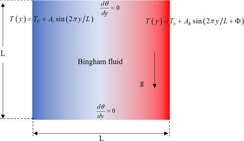
- Representative diagrams of the differentially heated cavity.
The momentum equations:
The Navier-Stokes equations system for this study is presented as follows (Sairamu et al., 2013).
The continuity formula:
Following
:
Following
:
The energy equation:
The above equations became dimensionless by introducing these variables.
The top and the bottom boundaries of the domain:
The vertical walls are exposed to sinusoidal temperatures:
,
,where
represents the amplitude of the sinusoidal temperature. The bottom of the cavity represents the lowest point, while the highest point is located at the top, with
and
. These types of boundary conditions are not defined in the software for this reason we have developed two user-defined functions written in
language to model the problem. The thermal transfer rate is analysed by the parameter Nusselt quantity. The overall thermal flow rate for the entire enclosed space is the summation of the average Nusselt quantities alongside the heated halves of the two vertical sidewalls, as mentioned by the average Nusselt quantity:
The Nusselt number is computed for the investigated status to observe when rheological behavior leads to an improvement or degradation in heat transfer rate.
The Herschel-Bulkley model is controlled by the subsequent expressions:
The Bingham model is regulated by the next formulas:
Dimensionless Rayleigh number
Dimensionless Grashoff number:
Dimensionless Prandtl number
Dimensionless Bingham number:
3 Numerical methods
The numerical simulation is provided with the help of the commercial CFD software FLUENT. The governing equations are resolved to employ a finite volume approach established on the SIMPLEC (Semi-Implicit Method for Pressure Linked Equations-Consistent) methodology, which is a modified variation of the SIMPLE algorithm, is a mathematical calculation process that has been widely employed in the area of computational fluid dynamics to solve the Navier–Stokes equations. This approach was developed in the 1980 s to focus on the given boundary constraints. The equations are discretized by applying the second-order upwind differencing approach. Finally, when the total of the residuals is smaller than 10-5, the convergence conditions for governing equations are satisfied.
3.1 Mesh test
The influence of the mesh on the results is tested and for this, three structured meshes
(40 × 40),
(80 × 80) and
(160 × 160) are used, however, the results obtained from the Nusselt number are presented in Table 1.
Mesh
Grids
40 × 40
80 × 80
160 × 160
1.5167
1.5264
1.5286
It is observed that the heat transference rate (Nusselt numbers) exhibits constant values. for the two meshes and . Nevertheless, the judicious choice of the mesh (6561 nodes, 6720 elements) is a good compromise between precision and the cost in CPU time.
3.2 Validation
To confirm the accuracy of our findings, we compare them with the results obtained in previous studies conducted by the references mentioned in the literature. (Danane et al., 2020; Sairamu et al., 2013) and (Santos et al., 2021) in Fig. 2. The numerical model in this study collaborates and the Nusselt is compared, which is a parameter that includes speeds and temperatures with the following correlation:
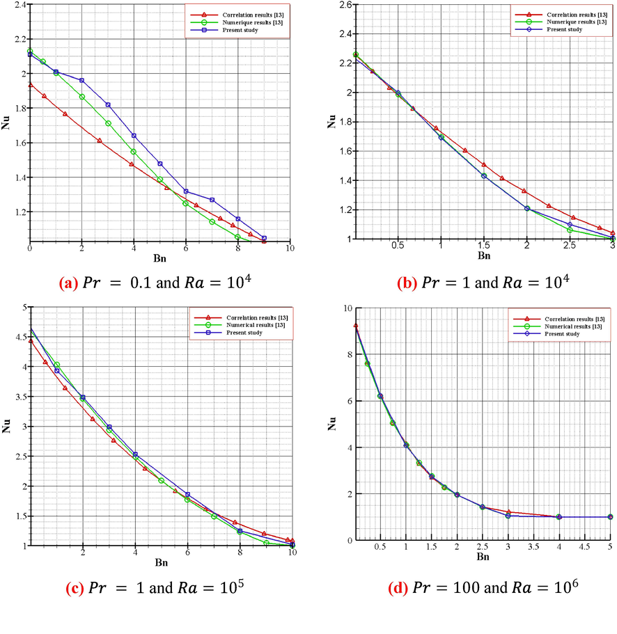
Comparison of the relationship provided in Eq. (13) with the computational results achieved and those of Ref. (Danane et al., 2020).
Nusselt numbers are compared and validated with results from Refs. (Hassan et al., 2020); (Turan et al., 2011) and (Turan et al., 2010), respectively as shown in Table 2, Figs. 3 and 4. An acceptable accord can be seen from the current outcomes and the ones described in Refs. (Hassan et al., 2020); (Turan et al., 2011), and (Turan et al., 2010).
1
3
6
9
18
27
Ref. (Hassan et al., 2020)
3.303
3.263
3.083
2.898
2.402
2.143
Present
3.305
3.265
3.083
2.900
2.403
2.140
Comparison of the numerical result obtained (o) with those of Ref. (Turan et al., 2011) (--) of the influence of the phase variation (
) on the mean Nusselt numbers for
.
Comparison of numerical results obtained (o) with those in Ref. (Turan et al., 2010) (--) of the influence of the phase change (
) on the mean Nusselt numbers for
.
4 Results and discussion
This part will be reserved for the two-dimensional model of the free convective flowing of a differential heated cavity. Rayleigh quantity , the Bingham quantity , the Prandtl quantity , the amplitude , phase difference , and flow index are varied to get the results.
4.1 Rayleigh number effect
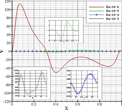
The dimensionless temperature and velocity distributions of non-Newtonian (the Bingham fluid) and the Newtonian fluid along the horizontal mid-plane are demonstrated in Figs. 5, 6, and 8, 9, separately, for different Rayleigh values. For
, the temperature outline is perfect linearly, and the rapidity at the vertical plane is negligible because the flow is very small. Since the effect of buoyancy is primarily related to the viscous effect. According to these conditions, heat transfer is entirely conducted through the cavity. At smaller Rayleigh numbers (
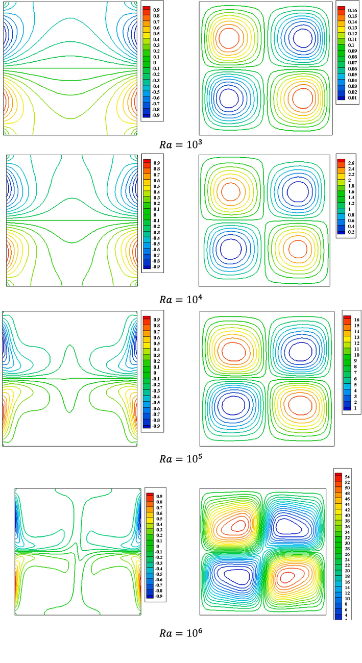
), convection is too weak, so thermal flow is controlled by thermal conducting mechanisms, as illustrated by the isothermal lines. when the Rayleigh quantity rises to
, the isotherm structures and the streamline structures begin to change for both Bingham and Newtonian fluids as shown in Figs. 7 and 10 respectively. We noted that the streamlines' structure is in the shape of four-spot cells with symmetries, approximately vertically and horizontally, however, these cells change and deform where the increment of the Rayleigh value. At this particular juncture, convectional heat is evidently initiated.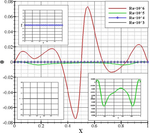
Bingham's dimensionless fluid temperatures when
,
,
, and
.
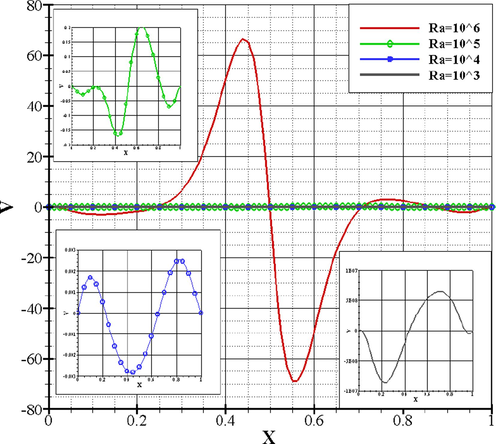
Bingham's dimensionless fluid velocities when
,
,
, and
.
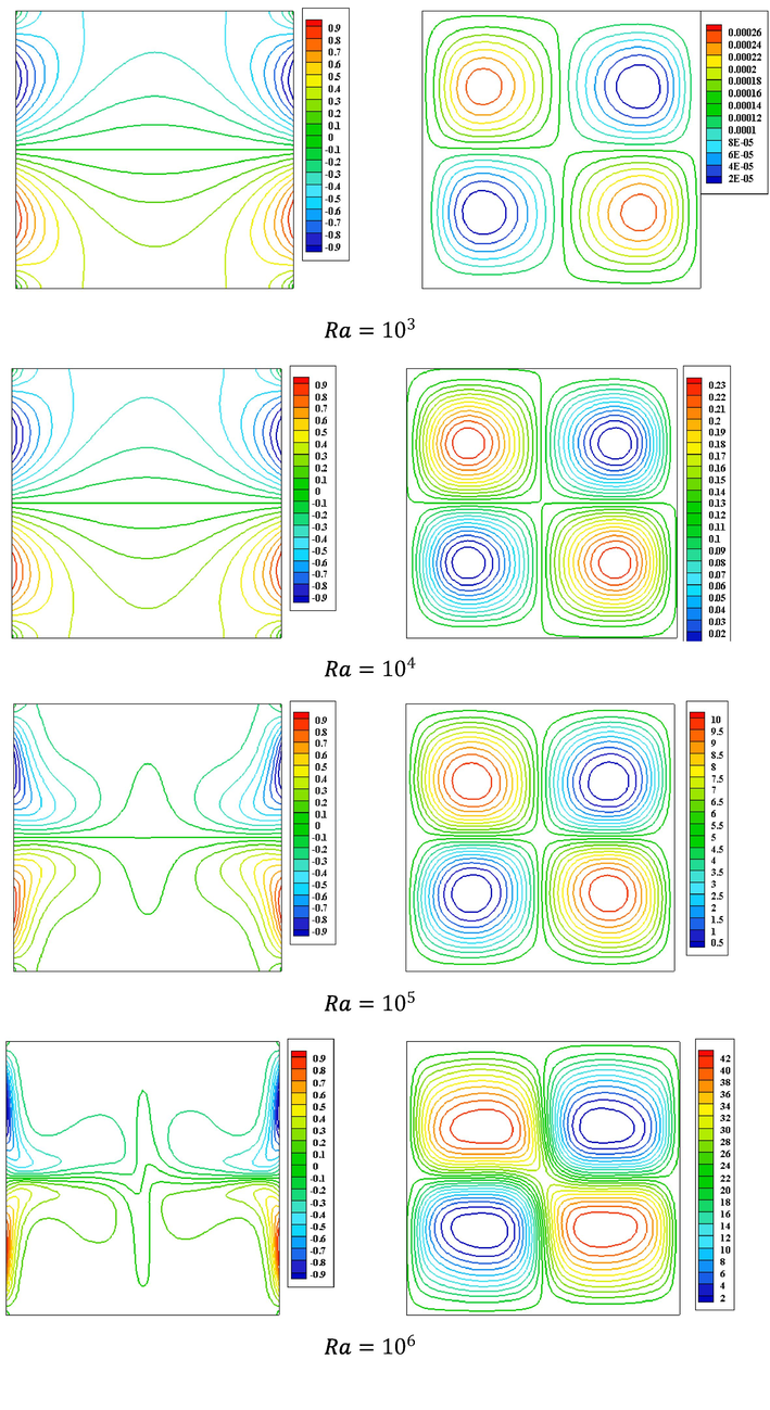
Isotherm contours (left) and streamline contours (right) of the Bingham fluid for
,
,
, and
.
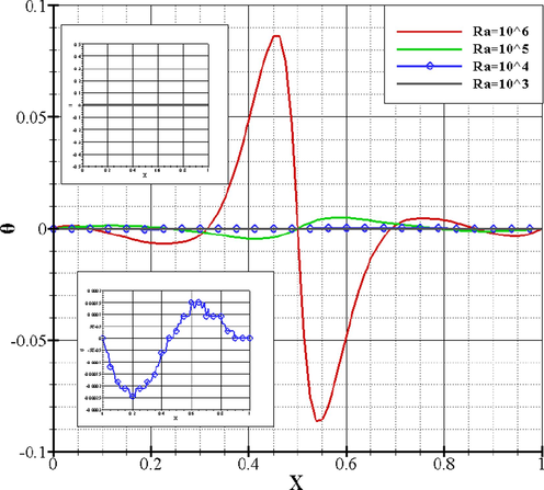
Dimensionless Newtonian fluid temperatures for
,
,
, and
.
Dimensionless Newtonian fluid velocities for
,
,
, and
.
Isotherm contours (left) and streamline Contours (right) of the Newtonian fluid for
,
, and
.
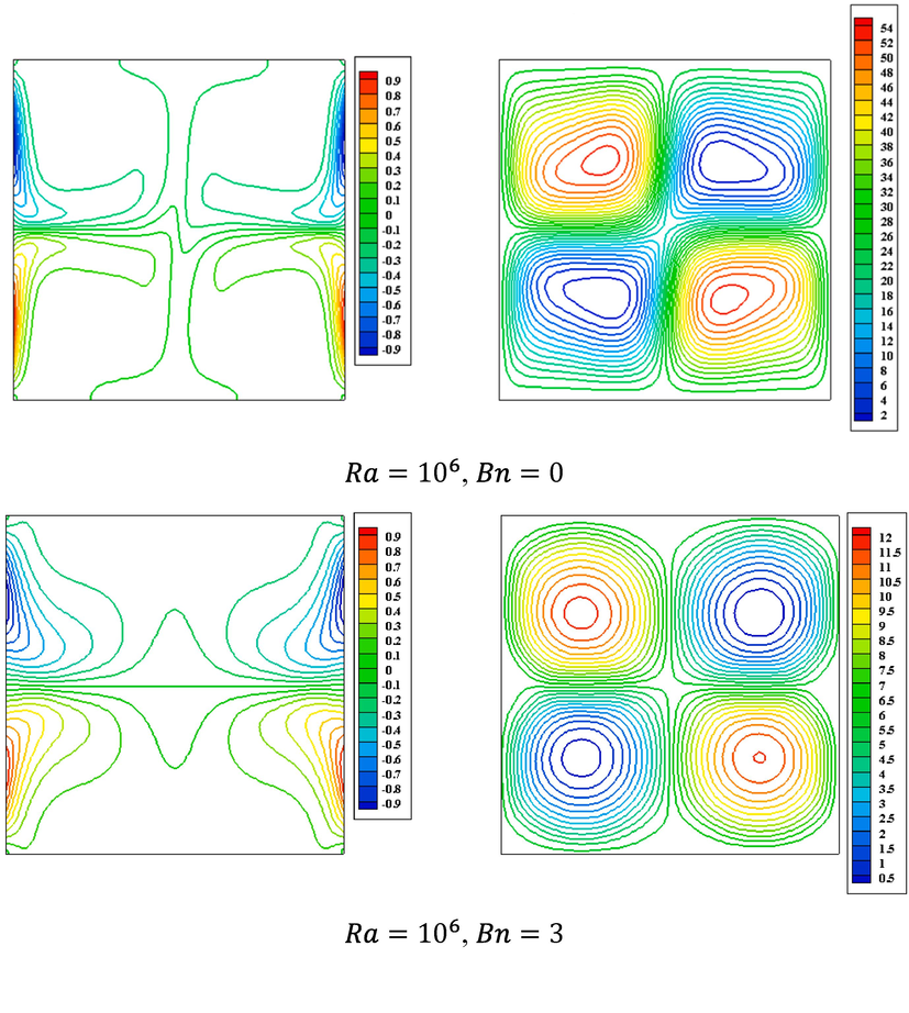
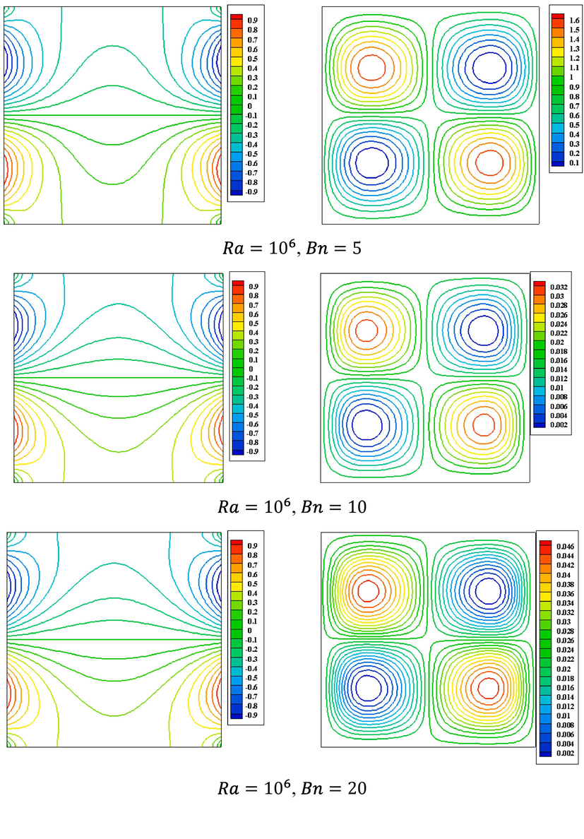
4.2 Bingham number effect
With higher plasticity values (
), the viscid power added easily affects the buoyancy power, and hence no fluxing is created in the cavity. This result is evident from Figs. 11 and 12, 14 and 15 where the influence of plasticity parameters (
) on the dimensionless temperature distributions and the velocity at the horizontal level are observed for
and
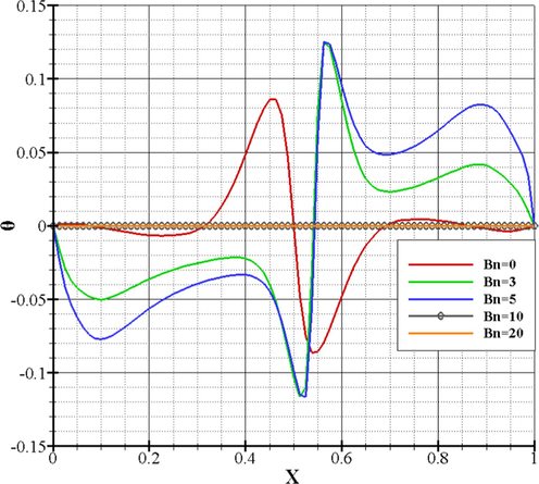
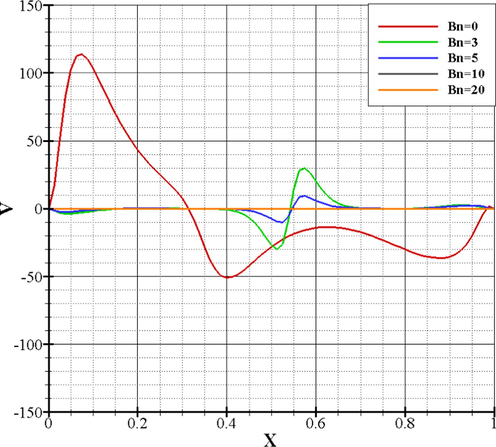
. It could be observed in Figs. 11 and 12, 14 and 15 For higher amounts of
, the temperature distribution becomes uniform, and the vertically element of the rapidity vanishes, under this situation, the thermal flow occurs entirely by conduction through the cavity. We add to this that the temperatures and velocities take a sinusoidal form depending on the nature of the boundary constraints.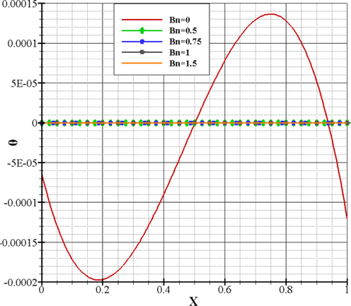
Bingham's dimensionless fluid temperatures for
,
,
, and
.
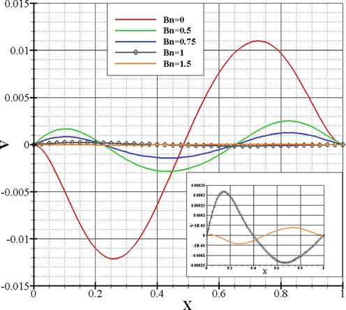
Bingham's dimensionless fluid velocities for
,
,
, and
.
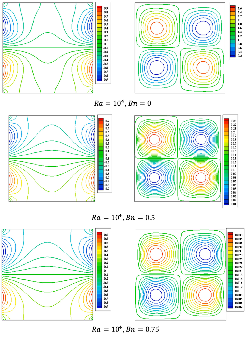
Bingham fluid isotherm contours (left) and streamline contours (right) when
,
, and
.
Bingham fluid isotherm contours (left) and streamline contours (right) when
,
, and
.
Bingham's dimensionless fluid temperatures for
,
,
, and
.
Bingham's dimensionless fluid velocities for
,
,
, and
.
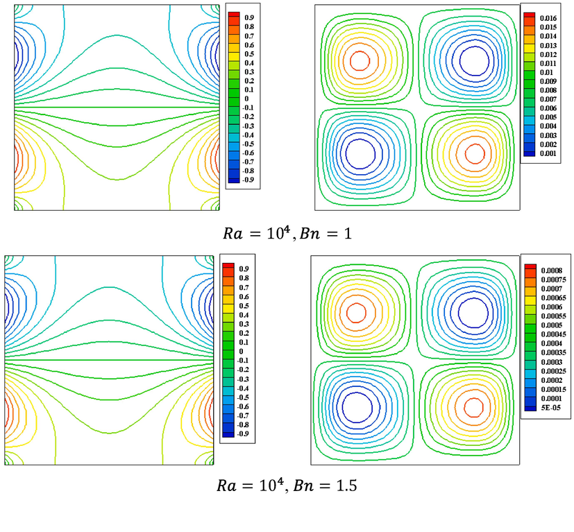
A better understanding of this behavior can be achieved by comparing the streamlined contours and dimensionless isotherms depicted in Figs. 13 and 16. For diverse amounts of
at
and
respectively. These figures reveal that the influence of convective within the cavity decreased with the growth of Bingham value and Bingham's fluid started to become like a solid. For
, the velocity of fluid decreases to such small amounts where for all reasonable determinations the liquid is mainly stagnating. In the absence of flux in the cavity, thermal flow occurs by conduction. Note that
for
and
for
.
The Bingham fluid isotherm contours (left) and streamline contours (right) when
,
, and
.
The Bingham fluid isotherm contours (left) and streamline contours (right) when
,
, and
.
4.3 Prandtl number effect
It is noticed that the contours of the isotherms which are indicated in Figs. 17 and 18 for
and
respectively, show that with the increase in
and
, the isotherms are grouped same cases for the boundary layers close to the two side walls. In this case, heat transport is accomplished entirely by conduction over the enclosure.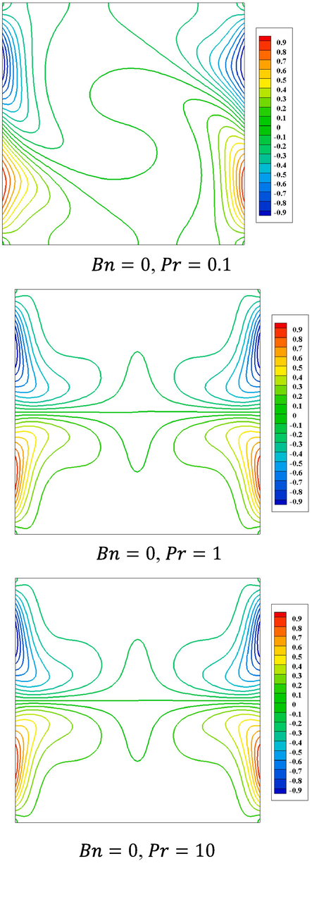
Contours of Newtonian fluid isotherms for
,
, and
.
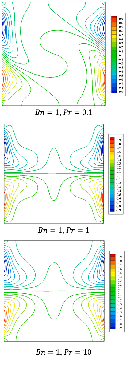
Contours of Bingham's fluid isotherms for
,
, and
.
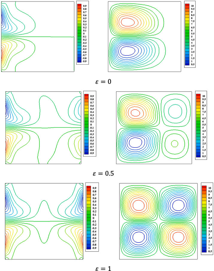
4.4 The impact of the phase variation
Fig. 19 illustrates the variants of the streamline contours and isothermal lines with a phase variation that varies from
to
. For a phase shift
, the streamlines have a structure with four cells which form a horizontal and vertical symmetry as long as the isothermal contours of the left side wall and that of the right are identical. For
the streamlines get a three-cell pattern with a single big diagonal cell and two small edge cells that are both the same size. The size of the upper edge cell grows larger as the phase difference rises. When
, the flowing system is two almost similar cells in the enclosed halves, and the bottom edge vanishes. The isothermal outlines along the left-side barrier are nearly retained after phase change modification, however, the isothermal patterns alongside the right-side barrier fluctuate. As a result, the heat transmission on the left-side barrier is maintained constant while it varies on the right-side barrier.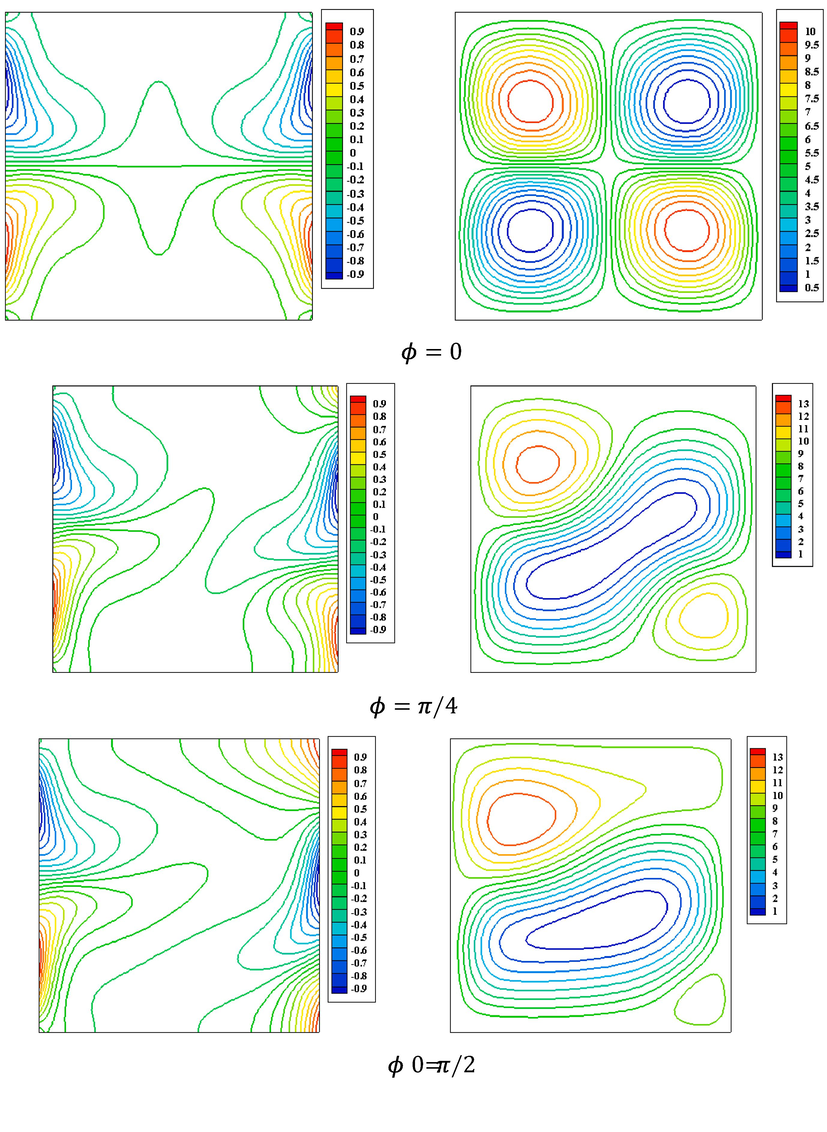
Isothermal contours (left) and streamlined contours (right) of the Bingham fluid when
,
,
, and
.
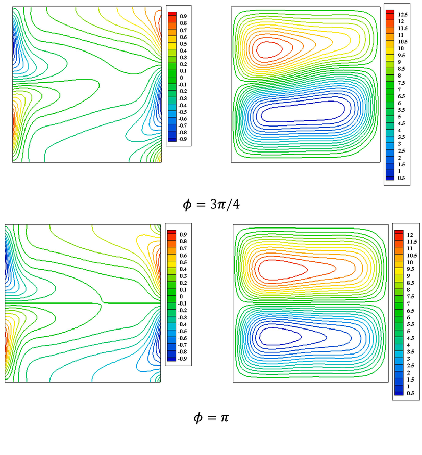
Isothermal contours (left) and streamlined contours (right) of the Bingham fluid when
,
,
, and
.
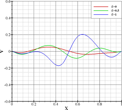
It has been noticed that the temperatures and the velocities indicated on Figs. 20 and 21 respectively, take sinusoidal forms according to the nature of the boundary conditions, it has also been observed that before
(left wall) the temperatures and the velocities decrease despite the increase in
but after
(right wall), the latter increase but negatively that we can explain by, since the temperatures and velocities increase with increasing phase shift
, we have the right wall which is more heated than the one on the left and this is due to the sinuses of the right wall which is greater than that of the left wall because the variation of
takes place on the right wall while
of the left wall is kept fixed, where the increase in the distribution of temperatures and velocities in the right wall is in a negative way which explains a depression, or that the flow increases with the increase in the phase shift but which is delayed and the convection is done in an anti-clockwise direction (from the right wall to the left wall). Finally, we noticed that
and
coincide.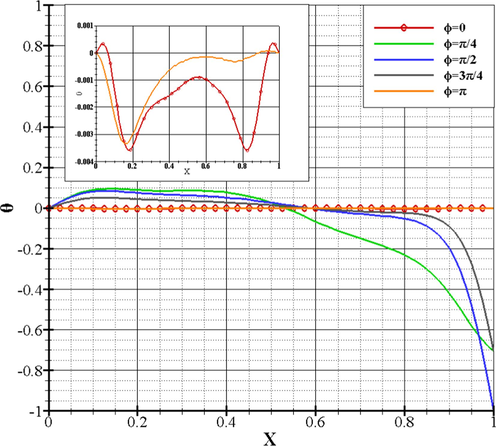
Bingham's dimensionless fluid temperature for
,
,
, and
.
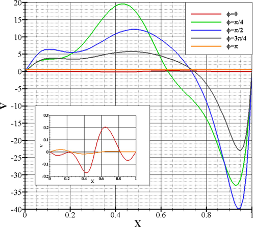
Bingham's dimensionless fluid velocity for
,
,
, and
.
4.5 The impact of amplitude
The streamlines and isothermal lines in the magnitude ratio example are exhibited in Fig. 22. The isothermal lines show that the temperature changes are mostly in a narrow surface close to the side wall left, while the streamlining shows that symmetrical cells are generated in the higher and lower centre of the cavity for (
).
Isotherms contours (left) and streamline contours (right) of the Bingham fluid for
,
,
, and.
Hence, heat transfer happens only on the left boundary wall. As the amplitude ratio rises to ( ), a four-cell flow is created inside the cavity, in addition, two subsidiary circulations are present near the right-sideways wall, in addition to the two primary circulations close to the left-side wall.
As a result, the isotherm along the left wall is remarkably similar to before, so the heat transference through the surface remains constant. However as observed, the temperature of the right wall is no longer consistent, and a few isothermal lines occur near the plane, resulting in poor heat transition. If
continues to increase, the flow structure changes. The two subordinate cells near the right-side wall change and form horizontal and vertical symmetry. Ultimately, it is remarked that the rise of
develops heat transference. It has also been noticed that the temperatures and velocities indicated in Figs. 23 and 24 respectively, increase with the increase in the ratio of the amplitude and take sinusoidal forms according to the nature of the boundary conditions.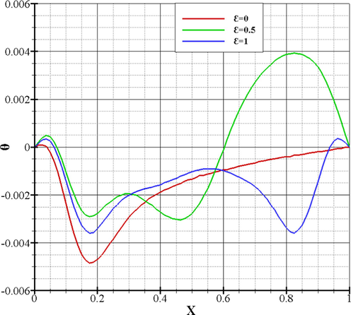
Bingham's dimensionless fluid temperature for
,
,
,
.
Bingham's dimensionless fluid velocity for
,
,
, and
.
4.6 Flow index effect
In Figs. 25, 26, and 27, streamlines and isotherms are shown for five values of
(0.3, 0.5, 0.75, 1.5, and 2.0). For
, it is noticed that the streamlines are of three-cell construction through one larger diagonal cell and two lesser edge cells of the same proportions, with increasing
the structure changes from three cells to four cells which forms a horizontal and vertical symmetry. As for the isotherms, their appearance changes with the increase in the flow index. We note that with this increase, the isotherms regroup which means slight lowness of the convection process.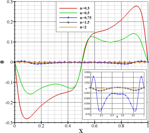
Bingham's dimensionless fluid temperature for
,
,
,
, and
.
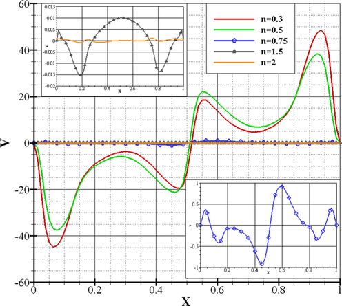
Bingham's dimensionless fluid velocity for
,
,
,
, and
.
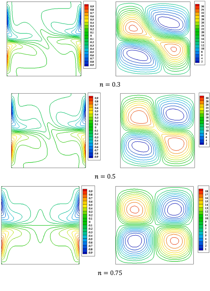
Bingham fluid isothermal contours of (left) and streamline contours (right) of the for
,
,
,
, and
.
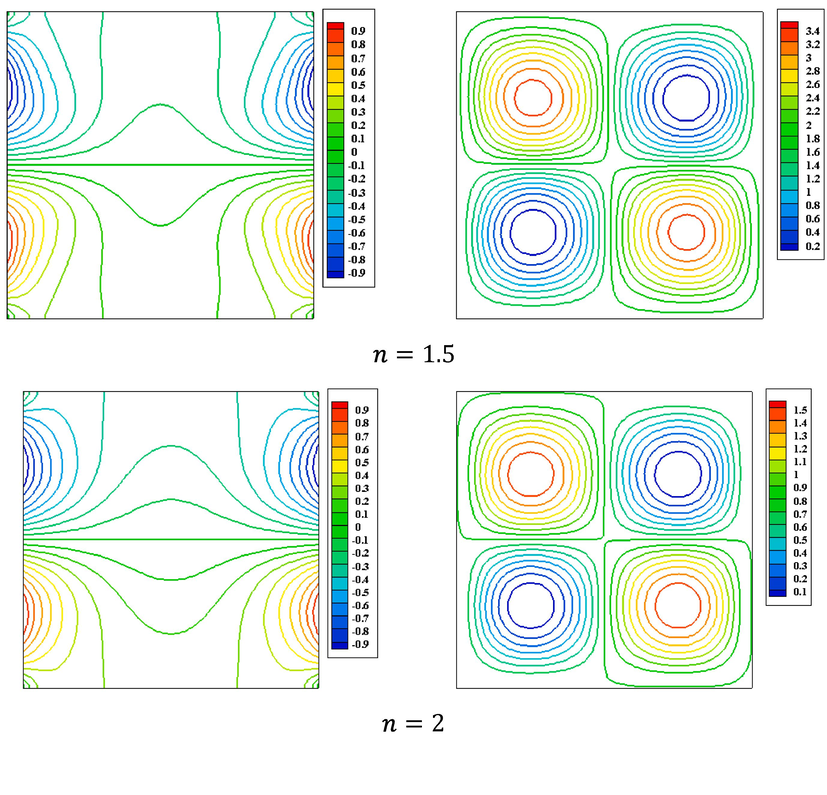
Bingham fluid isothermal contours of (left) and streamline contours (right) of the for
,
,
,
, and
.
This growth of the flow index has also influenced the vertical velocities which tend to decrease, and this is due to the increase in the apparent viscosity or quite simply that the fluid becomes viscous, as seen in Fig. 26, same observations for the temperatures which fall with the increase in n. It has also been noticed that the temperatures and velocities take sinusoidal forms depending on the boundary conditions.
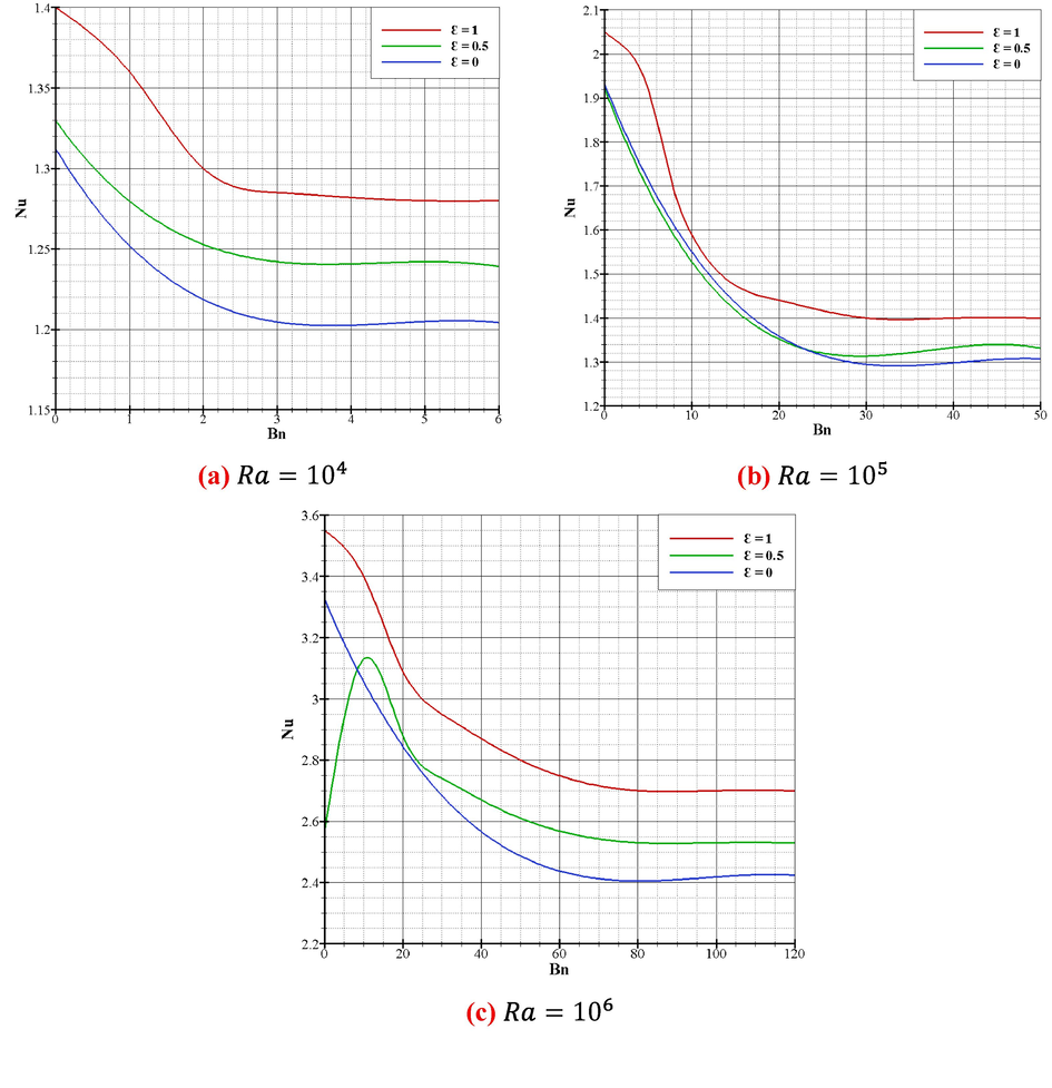
4.7 Effect of Nusselt number
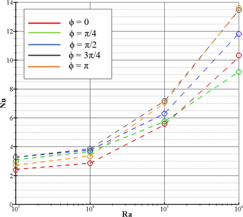
Fig. 28 depicts the fluctuations in the averaged Nusselt numbers that occur within the cavity in terms of the Rayleigh numbers for various levels of phase deviation. The remainder of the cavity's characteristics remain the same, with
,
. It has been discovered that the average Nusselt number, denoted by
, steadily increases whenever the Rayleigh numbers, denoted by
, go up for any given amount of phase variation value
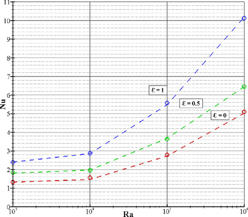
, denoted by. Fig. 29 displays the mean Nusselt numbers of changes of the cavity, denoted by
, in connection to Rayleigh quantity changes, denoted by
, for a variety of amplitude ratios
, denoted by. By increasing the Rayleigh numbers and maintaining the same amplitude ratio, the averaged Nusselt numbers will increase. Conversely, as the amplitude ratio grows from 0 to 1 for varying Rayleigh quantities, so does the average Nusselt quantity. The plot reveals that the heat transference increases with the amplitude ratio
and is higher for
than for
. It was discovered that the number of Nusselt decreased as the number of Bingham increased, especially at high Bingham numbers, since heat transmission was mostly accomplished by conduction. The regime dominated by conduction results in higher
values in exchange for increasing
values.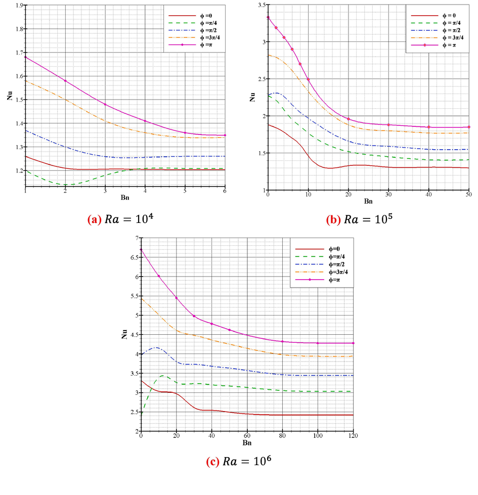
Influence of the phase variation
on the mean Nusselt numbers for
and
.
Influence of the amplitude ratios
on the mean Nusselt numbers for
and
.
5 Conclusions
This study relates a computational examination of the 2-D and 3-D free convective flowing of a viscoplastic fluid. The viscoplastic comportment is depicted by the Bingham prototype. The 3-D considered convection flowing is constrained in a cavity, subject to the horizontal temperature differences knowing that the horizontal sides are thermal isolated, and the vertical sides have two sinusoidal temperatures. The following conclusions can be drawn:
-
▪
For rising Rayleigh levels, the conducting dominated process comes at larger Bingham numbers.
-
▪
The Nusselt number decreases with improving Bingham quantity, For larger quantities of the latter, heat transfer primarily occurs through conduction. in contrast, the Nusselt of Newtonian and Bingham liquids increases with increasing Rayleigh values. Heat transference boosts as the amplitude ratio grows.
-
▪
The growth in the phase change indicates the growth in the heat transference, concerning the impact of the phase shift on the Nusselt numbers, the latter is always increased because of the number of Rayleigh boosts for all phase differences. It is noted that the thermal transition rate is enhanced for .
-
▪
As the amplitude ratio rises, heat transfer increases. We also found that the discrepancy of the average Nusselt related to the Rayleigh amounts, when the Rayleigh increased the Nusselt increased. The thermal flow rate for is greater than in the other situations.
-
▪
The increase in the flow index n slightly lowers the convection process and indicates an expansion in the apparent viscosity or simply that the liquid becomes viscous.
6 Authors' contributions
MB, KM, and DB formulated the problem. MM, KB, MI, WJ, and MRE solved the problem. WJ, MRE, and SMED computed and scrutinized the results. All the authors equally contributed to the writing and proofreading of the paper. All authors reviewed the manuscript.
CRediT authorship contribution statement
Brahim Mebarki: Conceptualization. Keddar Mohammed: Investigation, Writing – review & editing. Mariam Imtiaz: Writing – review & editing. Draoui Belkacem: Methodology, Software. Marc Medal: Formal analysis. Kada Benhanifia: Investigation. Wasim Jamshed: Software, Writing – original draft. Mohamed R. Eid: Formal analysis, Methodology, Writing – original draft. Sayed M. El Din: Writing – review & editing.
Declaration of Competing Interest
The authors declare that they have no known competing financial interests or personal relationships that could have appeared to influence the work reported in this paper.
References
- Natural convection for a Herschel-Bulkely fluid inside a differentially heated square cavity. Int. J. Mech. Energy (IJME). 2018;6(1):7-15.
- [Google Scholar]
- CFD analysis of two-dimensional non-Newtonian power-law flow across a circular cylinder confined in a channel. Chem. Eng. Commun.. 2012;199(6):767-785.
- [Google Scholar]
- A. Boutra, Y.K. Benkahla, D.E. Ameziani, N. Labsi, Etude numérique du transfert de chaleur pour un fluide de Bingham dans une cavité carrée en mode de convection naturelle instationnaire, CFM 2011-20ème Congrès Français de Mécanique, AFM, Maison de la Mécanique, 39/41 rue Louis Blanc-92400 Courbevoie, 2011.
- Simulations of Bingham plastic flows with the multiple-relaxation-time lattice Boltzmann model. Sci. China Phys. Mech. Astron.. 2014;57:532-540.
- [Google Scholar]
- Effect of backward facing step shape on 3D mixed convection of Bingham fluid. Int. J. Therm. Sci.. 2020;147:106116
- [Google Scholar]
- Natural convection of air in a square cavity: a bench mark numerical solution. Int. J. Numer. Meth. Fluids. 1983;3:249-264.
- [Google Scholar]
- Natural convection flows of a Bingham fluid in a long vertical channel. J. Nonnewton. Fluid Mech.. 2013;201:39-55.
- [Google Scholar]
- Natural convection of viscoplastic fluids in an enclosure with partially heated bottom wall. Int. J. Therm. Sci.. 2020;158:106527
- [Google Scholar]
- Natural convection problem in a Bingham fluid using the operator-splitting method. J. Nonnewton. Fluid Mech.. 2015;220:22-32.
- [Google Scholar]
- Agitation of complex fluids in cylindrical vessels by newly designed anchor impellers: Bingham-Papanastasiou fluids as a case study. Period. Polytech. Mech. Eng.. 2022;66:109-119.
- [Google Scholar]
- Double-diffusive natural convection and entropy generation of Bingham fluid in an inclined cavity. Int. J. Heat Mass Transf.. 2018;116:762-812.
- [Google Scholar]
- Lattice Boltzmann method for natural convection of a Bingham fluid in a porous cavity. Physica A. 2019;521:146-172.
- [Google Scholar]
- J.L.V. Ortega, Bingham Fluid Simulation in Porous Media with Lattice Boltzmann Method, Computational Fluid Dynamics Simulations, IntechOpen 2019.
- Natural convection from a circular cylinder in confined Bingham plastic fluids. Int. J. Heat Mass Transf.. 2013;60:567-581.
- [Google Scholar]
- A new design of a solar water storage wall: a system-level model and simulation. Energy Syst.. 2018;9:361-383.
- [Google Scholar]
- Natural convection of a viscoplastic fluid in an enclosure filled with solid obstacles. Int. J. Therm. Sci.. 2021;166:106991
- [Google Scholar]
- Laminar natural convection of Bingham fluids in a square enclosure with differentially heated side walls. J. Nonnewton. Fluid Mech.. 2010;165:901-913.
- [Google Scholar]
- Aspect ratio effects in laminar natural convection of Bingham fluids in rectangular enclosures with differentially heated side walls. J. Nonnewton. Fluid Mech.. 2011;166:208-230.
- [Google Scholar]
- On the onset of natural convection of Bingham liquid in rectangular enclosures. J. Nonnewton. Fluid Mech.. 2010;165:1713-1716.
- [Google Scholar]


