Comparing the modeling functions of hybrid nano-lubricant containing CuO and MWCNTs with standard quality measurement criteria to introduce the most optimal correlation function

1 Introduction

Today, nanotechnology has made great progress in various industries, including the automotive industry, because with the help of this technology, special things such as improving viscosity and reducing friction, etc., can be created in engine parts, which will suffer from defects with other methods. One of the main parts of the car that plays an important role in its movement is the car engine, which is very important due to its health. The engine plays an essential role in the movement of the car, from the fuel department to the transmission of energy or power to the wheels. The power of the engine is the result of the connection of its parts with each other (Vakili-Nezhaad and Dorany, 2009), but if there is friction between such parts, it means corrosion and shortens the lifetime of the parts. Therefore, experts in this industry have been looking for a way to reduce friction and increase engine life. Engine oil plays an important role in the moving parts of the engine. In addition to the lubrication of moving parts, engine oil should not lose its quality and efficiency under the influence of atmospheric conditions and face a drop-in efficiency. For this reason, experts are thinking of producing motor oils with more capabilities and efficiencies (Aghaei et al., 2017). Viscosity is one of the important indicators in choosing engine oil. Viscosity is the resistance of a fluid or liquid to movement or flow. Viscosity in liquids is due to the presence of intermolecular attraction that changes under the influence of temperature (Ghazvini et al., 2012). Viscosity has an inverse relation with the temperature variable, and this important principle should be considered in choosing a good engine oil. Lubrication of parts with oil starts from the time of starting the car, it is at this time that the engine oil must quickly lubricate all parts to avoid serious damage (Stanciu, 2017; Esfe and Arani, 2018). To prevent such problems and also to improve the viscosity of oils, researchers first used millimeter or micrometer-sized particles, which noticed sedimentation, low stability, and reduced viscosity changes, and looked for particles with smaller dimensions (Meybodi et al., 2016; Ahmadi et al., 2013). For the first time in 1995, Choi (Choi and Eastman, 1995) presented the idea of using particles less than 100 nm with high thermal conductivity (TC) and low volume ratio to normal fluids and preparing nanofluids (NFs) to improve viscosity and TC. NFs are a new generation of fluids that by adding oxide and non-oxide nanoparticles (NPs) and carbon nanotubes (CNTs) to engine oil have had a significant effect on improving the quality and viscosity of thermal oils (Saboori et al., 2017; Asadi et al., 2016). Viscosity is one of the most important dimensions of rheological behavior in the study of thermophysical properties of NFs, which can improve the performance and work efficiency of using smart fluids. In addition to engine oil lubrication, viscosity plays an important role to pumping power and pressure drop in heating systems (Bafrani et al., 2020). Also, NF viscosity affects the overall performance of the heat transfer system, which was worked on by Azimi et al. (Azmi et al., 2014). Various research was done in the field of the viscosity of NFs, but more research is still needed. In recent years, NFs have attracted the attention of many researchers (Du et al., 2020). The research group of Hemmat Esfe et al. (Esfe and Sarlak, 2017) evaluated the thermophysical properties of CuO-MWCNT hybrid NF (85 %-15 %)/10 W40 in SVF = 0.05–1 % and T = 55–55 °C. NF has shown non-Newtonian Bingham behavior at T < 45 °C. Finally, at T > 45 °C, a mathematical correlation with a second-order accuracy of 0.9846 was presented to predict the dynamic viscosity of NF. The result of this correlation shows that the predicted data are in good agreement with the experimental data. In another study (Alidoust et al., 2022), the relative thermal conductivity (RTC) for the SWCNT (15 %)-Fe₃O₄(85 %)/Water NF was investigated in different parameters such as temperature and SVF. The initial increase in TC for NF compared to water at a T = 30 °C and SVF = 0.03 % is equal to 0.9 %, but the highest value of RTC is reported as 32.20 %, which is a significant value. Besides experimental studies, response surface methodology (RSM) has been used as a mathematical method to predict TC. MOD and RTC sensitivity are applied to check the accuracy of predictions. As a result, the highest RTC sensitivity is reported at + 1.58 %. Hemmat et al. (Esfe et al., 2018) investigated the viscosity of the ZnO-MWCNT/10 W40 NF in a laboratory as a result of the parameters of temperature, SR and SVF. The results at a temperature between 5 and 55 °C and SVF = 0.05–1 % show that the behavior of the NF is a non-Newtonian behavior and the power-law index increases with the increase of the SVF. Chiam et al (Chiam et al., 2017) investigated the viscosity of Al₂O₃ NPs in EG/water base fluid (BF) in the temperature range of T = 30–70 °C and SVF = 0.2–1 %. The results show that viscosity decreases with the increase of the participation percentage of EG base fluid in NF. The highest increase in viscosity occurs in the combined ratio of EG/water (40:60) at T = 60 °C and SVF = 1 %, which is more than 70 %. Hemmat et al. (Esfe et al., 2018) investigated the dynamic viscosity of hybrid NF from different combinations of carbon nanotubes (CNTs) with different percentages of TiO₂ NPs in 10 W40 BF under the influence of temperature variables and different SVFs. Experimental results show that increasing the percentage of CNT has a significant effect on the non-Newtonian behavior of NF, and this increases the shear-thinning behavior of the composition. Jeong et al. (Jeong et al., 2013) studied the viscosity and TC of ZnO NPs on the effect of particle shape. First, the SVF and TC of ZnO NPs with almost rectangular and spherical shapes were investigated in SVF = 0.05–5 %. Hemmat et al. (Esfe et al., 2022) investigated the rheological behavior of MWCNT (25 %)-MgO (75 %)/SAE40 NF in T = 25–50 °C and SVF = 0.0625 to 1 % and SR = 666.5 to 7998 s⁻¹ experimentally. The results of evaluating the rheological behavior of NFs show that NFs exhibit non-Newtonian behavior. In addition today scientists and engineers use various statistical and numerical models to save money and time as well as speed up the solutions. In the last few years, computational methods and the use of RSM have attracted the attention of many researchers. Researchers use the RSM to predict experimental data and optimize response function models (Chu et al., 2021; Esfe, 2017; Khetib et al., 2021). Qualitative indicators of NF viscosity modeling using the RSM have attracted the attention of many researchers. Kazemi et al. (Kazemi-Beydokhti et al., 2013) investigated the TC of CuO/Water NF by seven important parameters (T, SVF, particle size, pH, NP density, elapsed time, and ultrasound time) in a laboratory manner. This study has used the factorial modeling method to evaluate the main effects and their interaction on the ratio of heat transfers with the factorial modeling method and three other tests for analysis of variance (ANOVA). By comparing the predicted data with the experimental data, it is in good agreement with the experimental data. Hemmat et al. (Esfe et al., 2017) used a factorial modeling method to investigate the TC of MgO/Water NF with the effect of temperature, SVF and NP diameter parameters. This evaluation was done in SVF = 0.01 to 0.03. Regression analysis shows that the laboratory data has a coefficient of determination value of R² = 0.9994. The results of this investigation show that the parameters (temperature, SVF and NP size) affect the TC. Malika et al. (Malika and Sonawane, 2021) prepared a hybrid NF based on montmorillonite clay in different ratios of NPs (Cu: Ni) through the hydrothermal process. RSM was used to investigate the photocatalytic decomposition of dye solution. Also, ANOVA was conducted to evaluate the impact of input parameters on changes in the response variable. In this research, the RSM was used to predict the viscosity of MWCNT (10 %)-CuO(90 %)/10 W40 HNL. First, different models were investigated to predict the viscosity of HNLs. Then, the comparison between different statistical models is presented according to quality indicators and the best correlation model is introduced. This study will be studied experimentally in Hemmat research group and will be presented at the right time.

2 Methodology

In this research, RSM was used to check the laboratory data. From 174 experimental data, different models and viscosity changes of MWCNT (10 %)-CuO(90 %)/10 W40 HNL were presented.

3 Results and discussion

3.2

3.2 Choosing the best model

In this part, to select the best model, the statistical parameters and accuracy graphs of the models were examined among different models. Statistical parameters that are accurate for different models including R-squared, Adjusted R², Predicted R² and Std. Dev. and the graphs of residuals versus Run, normal probability, Box-Cox and residuals versus actual were checked.

3.2.1

3.2.1 Examining the parameters related to the accuracy of the models

3.2.1.1

3.2.1.1 Interpretation of R-squared

Adjusted R-squared and predicted R-squared values are analyzed to evaluate the accuracy of the presented models. First, the R-squared values for different HNL viscosity models were checked. The closer the R-squared values are to 1, the higher the accuracy of that model. The values related to 2FI, Quadratic, Cubic, and Quartic models are presented in Table 5. As reported in Table 5, the values of all models are higher than 0.99, but the Quartic model has a higher accuracy than the rest of the models.

Table 5 R-squared for different examined models.

Source	2FI	Quadratic	Cubic	Quartic
R2	0.9327	0.9748	0.9972	0.9993

3.2.1.2

3.2.1.2 Values of Adjusted R²

Adjusted R² is a type of R-squared, which is the amount of change around the mean value. These values are set based on the number of model parameters compared to the number of design points. This parameter is shown in Eq. (6). In Table 6, the data values related to Adjusted R² are reported. These values are equal to 0.9302, 0.9935, 0.9968, and 0.9992 for different 2FI, Quadratic, Cubic, and Quartic models. As shown in Table 6, Adjusted R² values increase with increasing order of equations.

(6)

$$\mathit{Adj}.R^2=1-\left[\frac{\left(\frac{{\mathit{SS}}_{\mathit{residual}}}{{\mathit{df}}_{\mathit{residual}}}\right)}{\left(\frac{{\mathit{SS}}_{\mathit{residual}}+{\mathit{SS}}_{\mathit{model}}}{{\mathit{df}}_{\mathit{residual}}+{\mathit{df}}_{\mathit{model}}}\right)}\right]=1-\left[\left(\frac{{\mathit{SS}}_{\mathit{residual}}}{{\mathit{df}}_{\mathit{residual}}}\right)/\left(\frac{{\mathit{SS}}_{\mathit{total}}-{\mathit{SS}}_{\mathit{curvature}}-{\mathit{SS}}_{\mathit{block}}}{{\mathit{df}}_{\mathit{total}}-{\mathit{df}}_{\mathit{curvature}}-{\mathit{df}}_{\mathit{block}}}\right)\right]$$

Table 6 Adjusted R² for different examined models.

Source	2FI	Quadratic	Cubic	Quartic
Adjusted R2	0.9302	0.9935	0.9968	0.9992

3.2.1.3

3.2.1.3 Values of pred. R²

Predicted R² values are calculated from Eq. (7). It is a measure of how well the models predict the response value. Predicted R² values for different models are presented in Table 7. According to Table 7, model 4 has the highest value compared to other models and is close to 1, indicating the high accuracy of this model.

(7)

$$\mathit{Pred}.R^2=1-\left[\frac{\mathit{PRESS}}{{\mathit{SS}}_{\mathit{residual}}+{\mathit{SS}}_{\mathit{model}}}\right]=1-\left[\frac{\mathit{PRESS}}{{\mathit{SS}}_{\mathit{total}}-{\mathit{SS}}_{\mathit{curvature}}-{\mathit{SS}}_{\mathit{block}}}\right]$$

Table 7 Predicted R² for different examined models.

Source	2FI	Quadratic	Cubic	Quartic
Predicted R2	0.9255	0.9715	0.9963	0.9989

3.2.1.4

3.2.1.4 Values of Std. Dev

Std. Dev. means the square root of the residual mean square. The values of different models are shown in Table 8. The smaller this value is, the better this model is compared to other models.

Table 8 Std. Dev. For different models.

Source	2FI	Quadratic	Cubic	Quartic
Std. Dev.	42.63	26.29	9.13	4.62

3.2.2

3.2.2 Examining the graphs related to the accuracy of the models

The graph of residual values for different experiments is drawn in Fig. 1. In Fig. 1, the assumption of constant variance is tested. Random dispersion should be present in all graphs, and if there is a meaningful trend in each graph, more accurate evaluations are needed. Also, the accuracy of modeling is higher when the amount of data values are within the specified range. The reason for using the transfer function is because of the high variance values in the chart. According to the diagrams in Fig. 1, the diagram related to the Quartic model is more accurate than other models because it is in the specified range.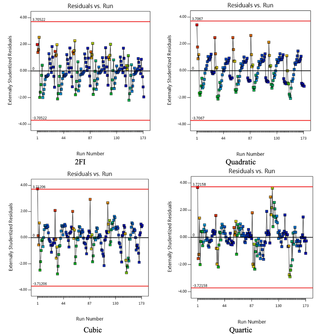

Close

Fig. 1

Residual values versus Run.

Export to PPT

The normal probability diagram for different 2FI, Quadratic, Cubic and Quartic models is drawn in Fig. 2. The purpose of drawing this graph is that the residuals follow the normal distribution of the data and are a straight line. Expect some scatter in the data, but if the data is s-shaped, the function is needed. As you can see in the graphs of Fig. 2, almost all of them are linear and there is very little deviation in the models.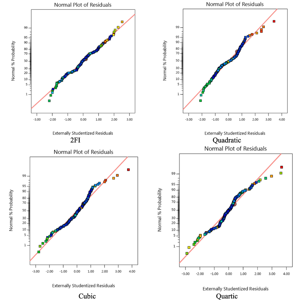

Close

Fig. 2

Normal distribution curve in terms of residual values.

Export to PPT

Fig. 3 shows the Box-Cox diagram for 4 models for MWCNT-CuO(10 %-90 %)/10 W40 HNL viscosity data. The Box-Cox plot provides a kind of guideline for choosing the correct transfer function. When the blue line is on point one, it means the 95 % confidence interval is around this lambda. According to the diagrams in Fig. 3, model 4 shows good behavior compared to the rest of the models, and the lambda line distance is in the lowest part of the curve.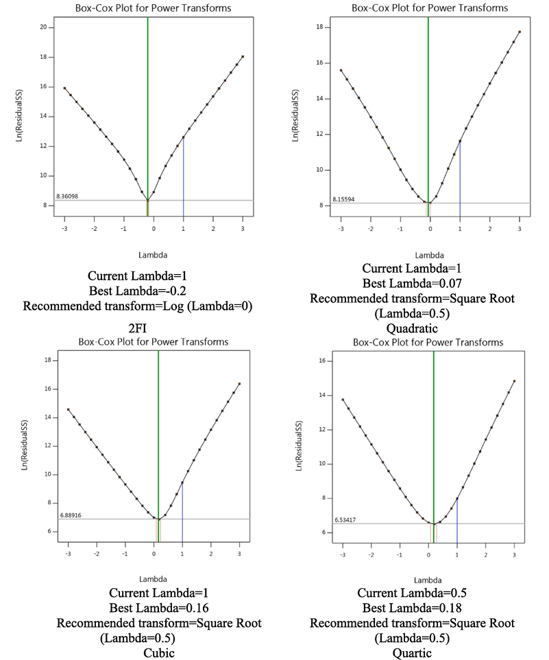

Close

Fig. 3

Box-Cox plots for determining Lambda values.

Export to PPT

Fig. 4 shows the predicted response values versus the actual values. With the help of this chart, it is possible to identify the big deviation in the predicted data compared to the real data. As the rank of the models increases, the accuracy of each model increases. According to Fig. 4, the Quartic model is well placed on the bisector line compared to other models, and this indicates the high accuracy of this model.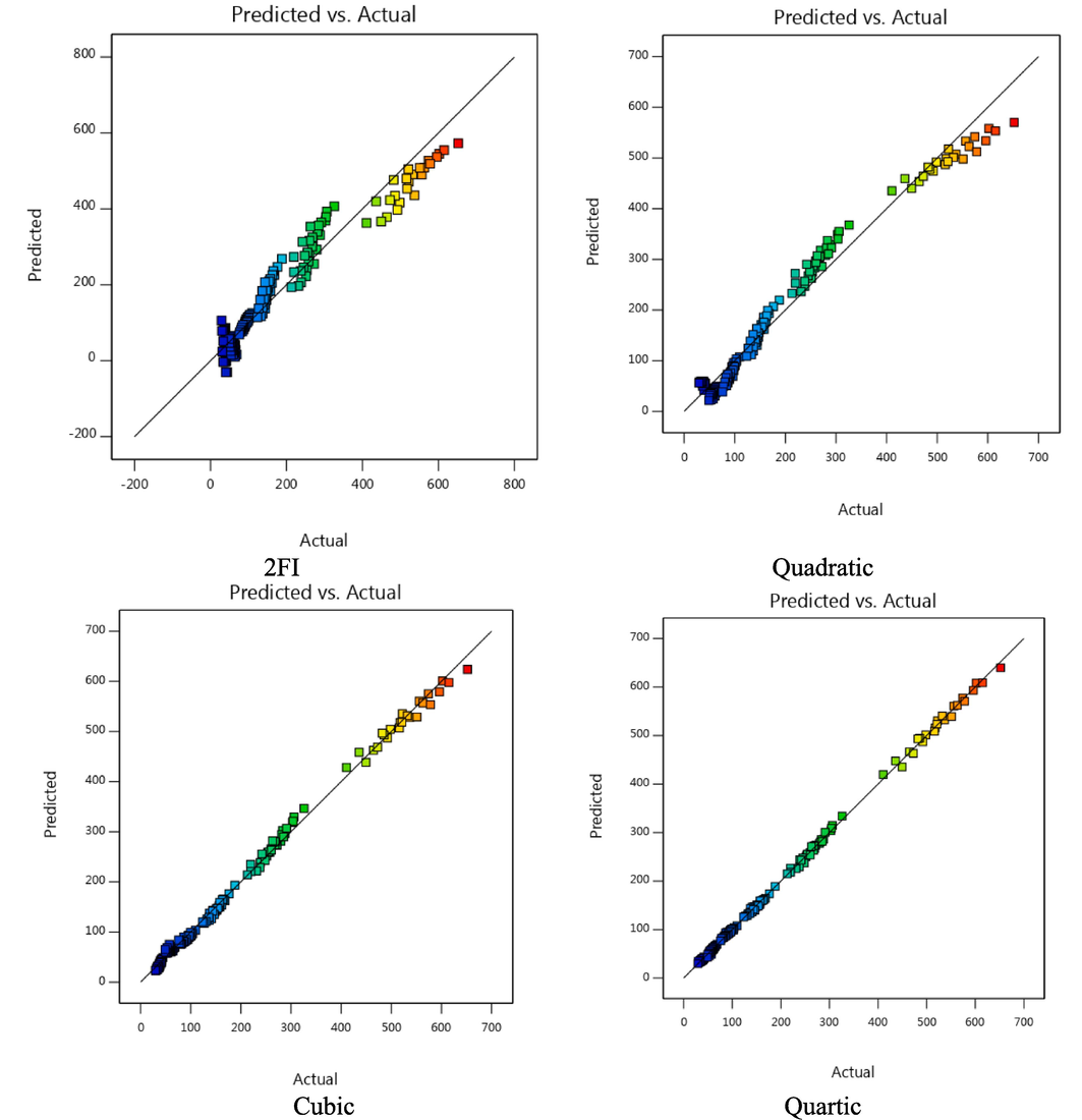

Close

Fig.4

Comparison of predicted and actual values.

Export to PPT

3.3

3.3 Viscosity changes in the selected model

The viscosity of the nanofluid is presented using the available data for the selected Quartic model. the viscosity at different points was calculated and evaluated its trend. The process of viscosity changes is drawn in Figs. 5 and 6. the trend of viscosity changes versus temperature and concentration is shown in Fig. 5. An increase in temperature has led to an decrease in the dynamic viscosity of the nanofluid. Viscosity changes in terms of temperature and SR for this selected model are plotted in the figure.Viscosity changes in terms of temperature and SR for this selected model are plotted in Fig. 6.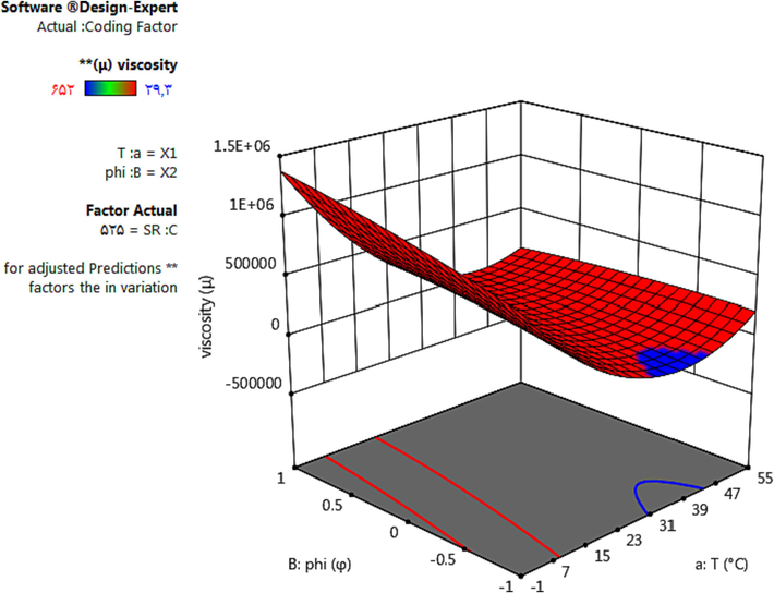

Close

Fig. 5

Changes in HNL viscosity versus T and SVF.

Export to PPT

Close

Fig. 6

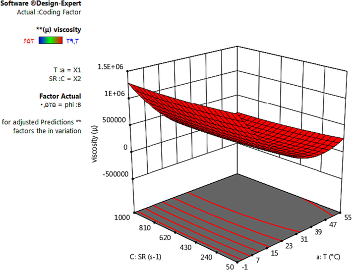
Changes in HNL viscosity in terms of T and SR.

Export to PPT

4 Conclusion

One of the best methods for estimating material properties is the RSM. In this research, the RSM was used to predict the viscosity of MWCNT (10 %)-CuO(90 %)/10 W40 HNL and the selected model among several models for HNL viscosity was presented. The analyzed models for this work include 2FI, Quadratic, Cubic and Quartic models. Statistical parameters and accuracy graphs were used to evaluate the models. Statistical parameters include Adjusted R², Predicted R² and Std. Dev. Each of them evaluated the accuracy of the models in a different way. It has been determined that the Quartic order model is more capable to other models (R-Squared = 0.9993). The comparison chart between the predicted data and the real data shows that the Quartic model is well placed on the bisector line and this shows the high accuracy of this model compared to other models.

References

- Experimental measurement of the dynamic viscosity of hybrid engine oil-Cuo-MWCNT nanofluid and development of a practical viscosity correlation. Modares Mechanical Engineering. 2017;16(12):518-524.
- [Google Scholar]
- Preparation and thermal properties of oil-based nanofluid from multi-walled carbon nanotubes and engine oil as nano-lubricant. Int. Commun. Heat Mass Transfer. 2013;46:142-147.
- Investigation of effective parameters on relative thermal conductivity of SWCNT (15%)-Fe3O4 (85%)/water hybrid ferro-nanofluid and presenting a new correlation with response surface methodology. Colloids Surf A Physicochem Eng Asp. 2022;645:128625
- The effect of temperature and solid concentration on dynamic viscosity of MWCNT/MGO (20–80)–SAE50 hybrid nano-lubricant and proposing a new correlation: An experimental study. Int. Commun. Heat Mass Transfer. 2016;78:48-53.
- Heat transfer and friction factor of water based TiO2 and SiO2 nanofluids under turbulent flow in a tube. Int. Commun. Heat Mass Transfer. 2014;59:30-38.
- On the use of boundary conditions and thermophysical properties of nanoparticles for application of nanofluids as coolant in nuclear power plants; a numerical study. Prog. Nucl. Energy. 2020;126:103417
- Thermal conductivity and viscosity of Al2O3 nanofluids for different based ratio of water and ethylene glycol mixture. Exp. Therm Fluid Sci.. 2017;81:420-429.
- Choi, S. U., & Eastman, J. A. 1995. Enhancing thermal conductivity of fluids with nanoparticles (No. ANL/MSD/CP-84938; CONF-951135-29). Argonne National Lab. (ANL), Argonne, IL (United States).
- Examining rheological behavior of MWCNT-TiO2/5W40 hybrid nanofluid based on experiments and RSM/ANN modeling. J. Mol. Liq.. 2021;333:115969
- An experimental investigation of CuO/water nanofluid heat transfer in geothermal heat exchanger. Energ. Buildings. 2020;227:110402
- Designing a neural network for predicting the heat transfer and pressure drop characteristics of Ag/water nanofluids in a heat exchanger. Appl. Therm. Eng.. 2017;126:559-565.
- An experimental determination and accurate prediction of dynamic viscosity of MWCNT (% 40)-SiO2 (% 60)/5W50 nano-lubricant. J. Mol. Liq.. 2018;259:227-237.
- A study on rheological characteristics of hybrid nano-lubricants containing MWCNT-TiO2 nanoparticles. J. Mol. Liq.. 2018;260:229-236.
- A novel study on rheological behavior of ZnO-MWCNT/10w40 nanofluid for automotive engines. J. Mol. Liq.. 2018;254:406-413.
- Experimental investigation of switchable behavior of CuO-MWCNT (85%–15%)/10W-40 hybrid nano-lubricants for applications in internal combustion engines. J. Mol. Liq.. 2017;242:326-335.
- Application of three-level general factorial design approach for thermal conductivity of MgO/water nanofluids. Appl. Therm. Eng.. 2017;127:1194-1199.
- Investigating the rheological behavior of a hybrid nanofluid (HNF) to present to the industry. Heliyon 2022e11561
- Heat transfer properties of nanodiamond–engine oil nanofluid in laminar flow. Heat Transfer Eng.. 2012;33(6):525-532.
- Particle shape effect on the viscosity and thermal conductivity of ZnO nanofluids. Int. J. Refrig. 2013;36(8):2233-2241.
- Experimental analysis of drag reduction in the pipelines with response surface methodology. J. Pet. Sci. Eng.. 2016;138:104-112.
- Identification of the key variables on thermal conductivity of CuO nanofluid by a fractional factorial design approach. Numerical Heat Transfer, Part b: Fundamentals. 2013;64(6):480-495.
- Competition of ANN and RSM techniques in predicting the behavior of the CuO-liquid paraffin. Chem. Eng. Commun. 2021:1-13.
- Statistical modelling for the ultrasonic photodegradation of rhodamine B dye using aqueous based bi-metal doped TiO2 supported montmorillonite hybrid nanofluid via RSM. Sustainable Energy Technol. Assess.. 2021;44:100980
- A novel correlation approach for viscosity prediction of water based nanofluids of Al2O3, TiO2, SiO2 and CuO. J. Taiwan Inst. Chem. Eng.. 2016;58:19-27.
- Improvement of thermal conductivity properties of drilling fluid by CuO nanofluid. Challenges in Nano and Micro Scale Science and Technology. 2017;5(2):97-101.
- Viscosity index improvers for multi-grade oil of copolymers polyethylene-propylene and hydrogenated poly (isoprene-co-styrene) Journal of Science and Arts. 2017;4(41):771-778.
- Investigation of the effect of multiwalled carbon nanotubes on the viscosity index of lube oil cuts. Chem. Eng. Commun.. 2009;196(9):997-1007.