

Translate this page into:
Development of advanced machine learning models for optimization of methyl ester biofuel production from papaya oil: Gaussian process regression (GPR), multilayer perceptron (MLP), and K-nearest neighbor (KNN) regression models
-
Received: ,
Accepted: ,
This article was originally published by Elsevier and was migrated to Scientific Scholar after the change of Publisher.
Peer review under responsibility of King Saud University.
Abstract
Data-driven machine learning (ML) methods are extensively employed for modeling and simulation of highly complicated processes. ML techniques confirmed their great predictive capability compared to conventional techniques for modeling and management of non-linear relationships between input and output parameters. Biofuels as renewable sources of energy are a significant potential alternative to fossil fuels. Due to the non-linearity and complexity of biofuels production processes and increasing energy conversion, accurate and fast modeling tools are necessary for design and optimization of these processes. Hence, in this research, ML modeling techniques were developed for simulation of biofuel production from energy conversion of Papaya oil through transesterification process. In order to simulate and optimize the content Papaya oil methyl ester (POME) production, Gaussian Process Regression (GPR), Multilayer perceptron (MLP), and K-nearest neighbor (KNN) regression models, as well as adaptive boosting for amplification, were employed. The temperature of reaction, catalyst quantity, time of process, and methanol to oil molar ratio were considered as the inputs of models while the POME yield was the model output. The obtained results showed that the R2-score of 0.988, 0.993, and 0.994 were obtained for Boosted MLP, Boosted GPR, and Boosted KNN, respectively, which demonstrate the high predictive ability of these models. Also, the RMSE metric error rates of 9.8071, 4.8150, and 6.5180 corresponded to Boosted MLP, Boosted GPR, and Boosted KNN, respectively. We examined performance using another metric, MAE: 8.38008, 2.3184, and 5.21954 errors were observed for Boosted MLP, Boosted GPR, and Boosted KNN, respectively. The optimized POME production yield of 99.89% was observed at temperature of 62.5 °C, 6.47 min of reaction, catalyst quantity of 0.8125 wt% and methanol to oil molar ratio of 10.33. The obtained results of this study show that the ML techniques are highly recommended for prediction of biofuels production as cost and time saving methods.
Keywords
Papaya oil methyl ester (POME)
Computation
Biofuel
Machine learning

1 Introduction
Currently, more than 80% of the energy requirements are supplied by fossil fuels all over the world (Johnsson et al., 2019; Abas et al., 2015). Fossil fuels like natural gas, coal, and petroleum have some disadvantages that limited their usage (Aghbashlo et al., 2021). Not only the amount of these non-renewable energy resources are gradually reduced but also the emissions of greenhouse gases lead to the global temperature rising (Deng et al., 2020; Shine et al., 2005). Therefore, there has been a large deal of attention to alternative energy resources. Biofuels, especially the biodiesel (fatty acid methyl ester (FAME)) have been used as a good alternative because of advantageous like being non-toxic, renewable, eco-friendly and biodegradable (Chopade et al., 2012; Knothe, 2009; Ramírez-Verduzco et al., 2012). These promising fuels can be produced in a transesterification reaction of a triglyceride with an alcohol, which is catalyzed by a catalyst. Biofuels can be produced from different renewable oil sources such as animal fat, and vegetable oil (palm, papaya, corn…) (Liu and Zhang, 2023; Kamal Abdelbasset et al., 2022; Sumayli and Alshahrani, 2023). The global production of Papaya is at over 10 million tons per year, therefore, underutilized seed oil from Papaya can be a very good source for biofuel production (Agunbiade and Adewole, 2014. 2014.; Fuentes and Santamaría, 2014).
Different homogeneous and heterogeneous catalysts can be used in this process. Although homogeneous catalysts are more active, but they are not very useful due to problems like separation complexity and equipment corrosion (Liu et al., 2012; Tariq et al., 2012; Georgogianni et al., 2009). In comparison, heterogeneous catalysts are nontoxic and can easily separate from the reaction media. Apart from the type and amount of catalysts, different parameters affect the yield of transesterification process such as temperature, pH value, time of reaction and the methanol to oil ratio (Pardal et al., 2010; Sinha et al., 2008; Leung and Guo, 2006). Due to the nonlinearity and complexity of these processes, from physical and chemical point of view, an accurate, fast, and efficient modeling approach is required for design, control, and optimization of these systems (Mackenzie, 2015; Saldana et al., 2012; Weichert et al., 2019; Zhang et al., 2020).
Data-driven machine learning (ML) methods can be useful technique for modeling and optimization of complex, multivariate, and nonlinear systems which effectively reduce the quantity of tests and the overall time and cost of processes. ML is a collection of tools and techniques that automatically discover patterns from data with no assumptions about the data's structure. Neural networks, linear models, support vector machines, decision trees, and randomized trees are examples of ML approaches which had been used for data prediction in many different areas. One of the strengths of machine learning is that its strategies can develop non-linear correlations in data and interactions between predictors. One fundamental application of machine learning is regression tasks, and such a problem has been defined in this study (Senders et al., 2018; Cherkassky and Ma, 2003). Adaboost is a boosting model as a subcategory of ensemble model, like AdaBoost (Hastie et al., 2009) and gradient boosting (Friedman, 2001), which are built on an ensemble of weak estimators that are systematically appended to the ensemble (e.g., Neural networks, decision trees or other models). A weighted average of all the base estimator’s outputs was used to estimate what kind of result to expect. All of the remaining training samples are used to train the weak learners that have gone before it, and the weighted average of all of their outputs is used to teach them. The updated prediction error of the developed model is calculated after incorporating each weak learner in order to determine the weight coefficient given to each weak learner, which represents the contribution of that base learners to the final prediction. (after adding the weak learner) (Friedman, 2001). A Gaussian Process (GP) is a random variable set where some of them follow Gaussian distributions that are integrated together (Sumayli and Alshahrani, 2023; Grbić et al., 2013). Gaussian Process (GP) is commonly used as a fundamental stochastic process in geostatistics. It is used to directly represent Gaussian data and also serves as a base for non-Gaussian methods like linear regression models. GP regression is known for being both easy to implement and highly accurate with high generality for small datasets (Rasmussen, 2003; Daemi et al., 2019; Wang et al., 2019). MLPs are the most commonly employed model of neural networks for making predictions in the paradigm of supervised learning (Prechelt, 1996). The discussed neural network structure is a crucial type among various artificial neural networks. It is comprised of multiple neuron units, where each unit serves a distinct function. In contrast, a huge number of linked neurons can solve nonlinear and challenging problems. It was typically composed of input, output, and hidden layers. Through adjustment of the parameters and weights, these models can classify how inputs impact the outputs of the model (Zahavi and Levin, 1997). The kNN method is a type of supervised learning approach. In supervised learning, a function (the learner) is inferred from training data, which consists of a collection of examples (data points) (Bishop, 2006). Every individual data point comprises of an input vector (instance) along with the corresponding intended output value. The learner attempts to accurately identify the output for unseen cases after learning from the training set (Sumayli and Alshahrani, 2023).
In this study, the transesterification process for production of biofuel from non-edible Papaya oil was analyzed using machine learning method. The effect of different operating factors including methanol to oil molar ratio, the reaction temperature, time of process, and catalyst amount were evaluated on the production Papaya oil methyl ester (POME) efficiency. Three different models (MLP, KNN, and GPR) were used for modeling and simulation of this process. Previous study indicated that these models are great tools for biodiesel optimization (Sumayli and Alshahrani, 2023). Here, the models are boosted compared to the neat models to implement them for the process optimization. Also, the Adaboost was performed to improve these modeling methods to better study the biodiesel production from Papaya oil from computational point of view. The obtained results were compared, and the optimum condition were evaluated for maximum production of biofuel.
2 Dataset of process
Here we used a dataset on biodiesel production with values of various operational parameters for predicting POME production yield. It is crucial to note that these values were chosen based on preliminary testing conducted prior to the major experiments as reported by the source of data (Nayak and Vyas, 2019). The data used in this study are the same as those used in previous studies such as (Nayak and Vyas, 2019). In this regression problem, four input variables were selected as follows: temperature (represented by X1), the catalyst amount (represented by X2), time (represented by X3), and methanol-to-oil molar ratio (represented by X4). Also, the only output of our regression problem is POME (Papaya oil methyl ester) yield (represented by Y) (Sumayli and Alshahrani, 2023). In this dataset, there are 30 data points, which are shown in Fig. 1, the distribution of input and output variables.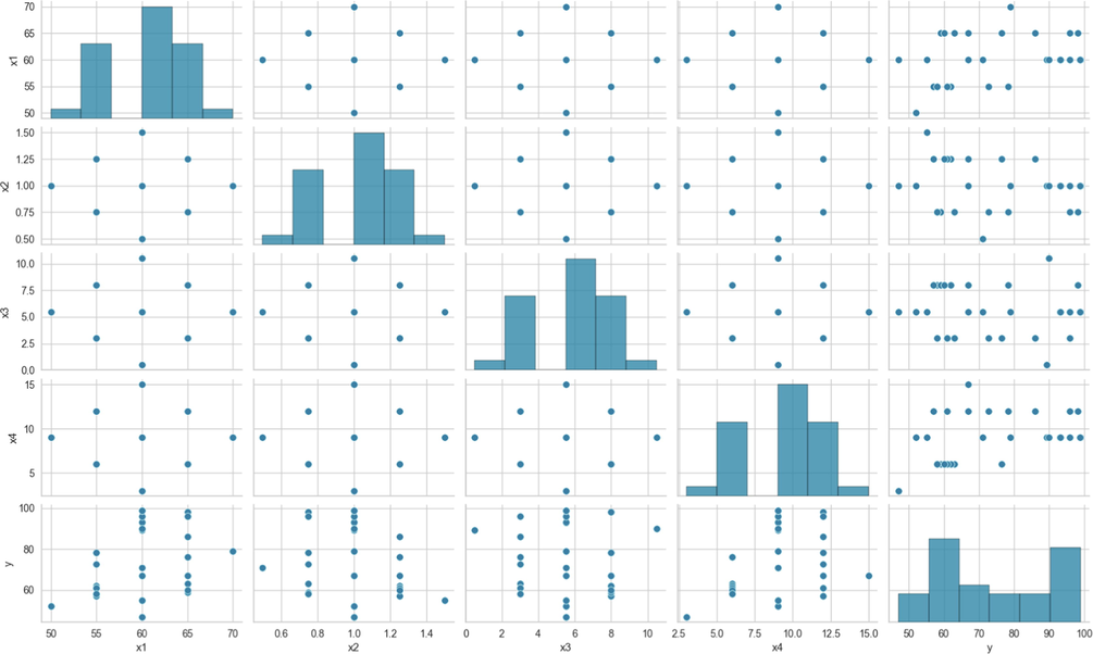
Scatter plot of data distribution.
3 Methodology
3.1 Gaussian process regression
The premise behind Gaussian processes regression (GPR) models is that neighboring observations should exchange data about one another. Gaussian processes are a way of defining a prior probability distribution over functions in function space. They extend the concept of a Gaussian distribution, with a covariance matrix and a mean vector, to the setting of functions. Gaussian processes are able to make predictions on new data without the need for a validation step, as they incorporate past information about the data and functional relationships. This makes Gaussian process regression models capable of finding the predictive distribution that corresponds to a new test input. The Gaussian process is just a multivariate Gaussian distribution (Rasmussen, 2003).
With respect to a given finite dataset consisting of n observations,
,
is the input vector of the ith instance and
denotes the observation value of the ith instance, respectively. The random variables
follow a joint Gaussian distribution, as depicted in equation (1):
Here,
denotes the mean function and
denotes the kernel function, both of which have the mathematical expressions in equations (2) and (3) (Huang et al., 2018):
A general model of the GPR problem (equation (4)) can be created by taking into account the noise in the measurements.
3.2 Multilayer perceptron
The MLP model, short for Multilayer Perceptron, is a sort of artificial neural network commonly employed for supervised learning tasks such as classification and regression analysis (Jain et al., 1996). The MLP algorithm has been widely applied to address various machine learning problems in different fields due to its ability to predict categorical and continuous variables with high accuracy (Soltani Fesaghandis et al., 2017). The MLP consists of layers of neurons, which are the primary components. Each layer is made up of clusters of neurons that take inputs from the layer below, process them using their activation function, and then transfer the output to the layer above (Kamal Abdelbasset et al., 2022; Noriega, 2005).
Neurons are arranged in layers in the MLP algorithm, where the input layer receives input, and the output layer generates output. To achieve optimal performance, certain parameters in a neural network must be adjusted, such as the solver functions, activation functions, and the size of hidden layers situated between the output and input layers (Kamal Abdelbasset et al., 2022). These are considered hyper-parameters and require fine-tuning. In the case of the MLP model with a single output and single hidden layer, equation (5) shows the output formula.
The predicted vector of the MLP model is represented by the symbol , and it is determined based on the input feature vectors, represented by xj. The weights linking the output layer to the hidden layer are represented as w(2), whereas the weights for the inputs linked to the hidden layer are indicated by w(1). The output layer utilizes an activation function labeled as δ2. Also, m and n are the count of instances and characteristics in the dataset correspondingly (Zhou et al., 2018). Neurons in the hidden layer are activated by the δ1 activation function, and the b(1) and b(2) symbols stand for the bias vectors used in the hidden layer and output layer, respectively. (Yang et al., 2008).
Changes are made to the weights between each link in a neural network to make it more accurate at predicting what will happen. Backpropagation and batch gradient descent, two popular learning methods, are used during training (Hecht-Nielsen, 1992).
3.3 K-nearest Neighbor
The K-Nearest Neighbors (KNN) regression model is an easy to understand method and utilizes the K nearest data points (most similar in input features) in the training dataset to estimate the value of a new observation. KNN regression is commonly used in a variety of applications, such as predicting stock prices, estimating housing prices, and forecasting weather patterns (Naghibi and Dashtpagerdi, 2017).
The KNN regression model operates by determining the distance between a new observation and all the observations present in the training data. The most common distance metric used is the Euclidean distance, which is calculated as displayed in equation (6).
Where, p stands for the count of input features, xik denotes the value of the kth input feature for the ith observation, and xjk stands for the value of the kth feature for the jth observation.
Once the distances are calculated, the KNN algorithm selects the K neighbors that have the shortest distances. The predicted value of the new observation is then calculated as the average (or median) of the target variable values of these K nearest neighbors.
One of the main advantages of KNN regression is its simplicity and interpretability. However, selecting a suitable value for K is crucial, as choosing too small or too large values may result in over-fitting or under-fitting, respectively. Furthermore, the performance of KNN regression may suffer in high-dimensional data or when the data has a complex structure (Bishop and Nasrabadi, 2006).
3.4 Adaptive boosting
As previously stated, the AdaBoost (Schapire, 2013) algorithm is the most commonly used ensemble learning algorithm. AdaBoost's distinguishing feature is that it builds a weak estimator using the initial training data, then modifies the training data distribution depending on prediction performance for the next round of weak estimator training. It's worth noting that in the next step, the training samples with low forecasting performance in the prior step will be given greater attention. Finally, the weak estimators are combined with a strong estimator using varied weights. The following is a description of the mathematical basis and implementation method. Both classification and regression can be done with AdaBoost. In the context of a general regression task, the training data set
can be written as shown in equation (7) (Strecht et al., 2015):
Then, using some special learning techniques, it may be utilized to train a weak estimators (or weak estimator) G(X), and the relative prediction error ei on each sample input can be represented in equation (8):
4 Results and discussions
Now, after reviewing the essential hyper-parameters of boosted models, the final findings are generated and analyzed. The effectiveness and accuracy of each model was evaluated according to statistical factors. The coefficient of determination (R2, equation (11)), mean absolute error (MAE, equation (13)), and root mean square error (RMSE, equation (12)) can be obtained as the following equations (Reiff, 1990; De Myttenaere et al., 2016; Karch and van Ravenzwaaij, 2020; Pelalak et al., 2021):
To fine-tune the hyper-parameters of the chosen algorithms, their various combinations were examined, resulting in approximately 2,000 individual runs of these values being optimized. Table 1 outlines the final set of hyper-parameters that were selected for the models. The term “number of estimators” in this table refers to the maximum number of base estimators at which boosting is ended. In the event of a perfect fit, the learning operation is terminated early, and each regressor weight at each boosting iteration is what is meant by learning rate. A faster learning rate boosts each regressor's contribution. Another parameter of adaptive boosting is loss function. To modify the weights after each boosting iteration, the loss function comes into play.
Models
Number of estimators
Loss function
Learning rate
Base Model Parameters
Boosted MLP
40
linear
0.12
Size of Hidden layers = 217
solver='lbfgs'
activation='relu'
tol = 0.0254
Boosted GPR
60
square
0.80
alpha = 4.468e-07
Num of restarts optimizer = 3
Boosted KNN
11
exponential
0.76
Number of neighbors = 3
weights='distance'
algorithm='brute'
Also in this table, for MLP model hidden layer sizes represent the number of neurons in the hidden layers and the hidden layer's activation function is set to 'relu' which returns f(x) = max (0, x) when the rectified linear unit function is used. In addition, the solver for weight optimization in boosted MLP decided to be ‘lbfgs’ which is an optimizer belongs to the category of quasi-Newton methods. The alpha value chosen for GPR is 4.468e-07, and the optimizer is restarted three times to obtain the kernel's parameters that maximize the log-marginal likelihood. In the final model, the number of neighbors for KNN was three. In addition, the model will perform a brute-force search to determine the nearest neighbors and the 'distance' weight function will be used in prediction. In the context of the algorithm being discussed, 'distance' refers to the manner in which points are given weight, which is based on the inverse of their distance. This means that points that are closer to a query point will have more of an impact than points that are farther away.
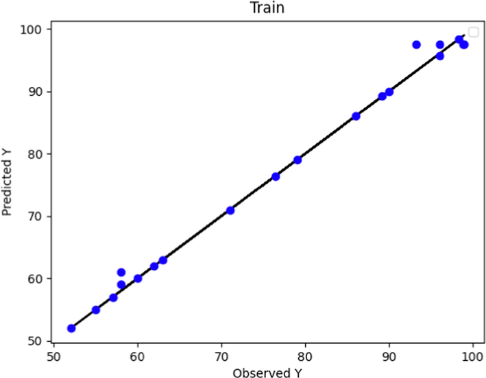
The observed and predicted POME values according to the Boosted MLP method for test and predicted data are depicted in Figs. 2 and 3, respectively. The boosted MLP model has shown high score and accuracy in the learning phase. The same thing can be seen in Fig. 3, so that in this diagram, most of the data points in the learning phase are completely on the line graph. However, in the test phase of this model, the distance between the predicted values and the actual values has increased to some extent, which is clearly shown in Fig. 2.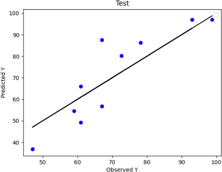
Predicted and Actual POME values comparison using Boosted MLP Model (test data).
Predicted and Actual POME values comparison using Boosted MLP Model (train data).
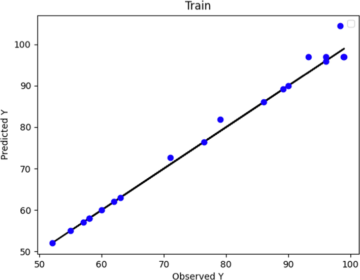
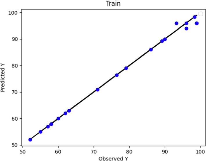
Similarly, the observed and predicted POME values according to the Boosted GPR method for test and predicted data are displayed in Figs. 4 and 5, respectively. For Boosted GPR model as shown in Fig. 5, the learning step is performed with high accuracy. Compared to the same figure for the boosted MLP model (Fig. 3), the learning steps of both models had a large extent. Although in both models the in training step the predicted and test data are close to each other, the boosted GPR model showed a more accurate learning phase. The subject is more different than the test diagrams in Fig. 2 and Fig. 4. The boosted GPR model made a more accurate prediction in the test phase and the deviation of the values (Fig. 4) was much less.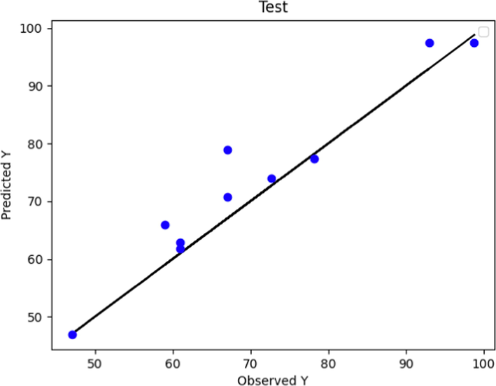
Predicted and Actual POME values comparison using Boosted GPR Model (test data).
Predicted and Actual POME values comparison using Boosted GPR Model (train data).
Figs. 6 and 7 depict the predicted and actual POME values using the Boosted KNN method for test and predicted data, respectively. By comparing the KNN model to the prior two models (Figs. 3 and 5), Fig. 7 shows that the KNN model, after being trained, achieves higher accuracy in terms of observed and predicted values. However, upon comparing Fig. 6 and Fig. 4, it can be inferred that the Boosted KNN method performed inferiorly during the test phase as compared to the boosted GPR.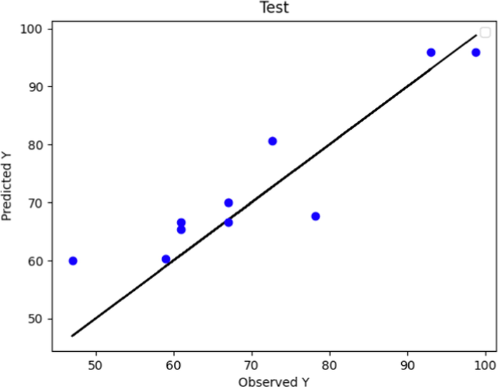
Predicted and Actual POME values comparison using Boosted KNN Model (test data).
Predicted and Actual POME values comparison using Boosted KNN Method (train data).
Table 2 reports the calculated values of R2, RMSE, and MAE for Boosted MLP, Boosted GPR, and Boosted KNN models. As can be seen in this Table, the regression coefficient for Boosted MLP, GPR, and KNN models were attained as 0.9882, 0.9938, and 0.9948, respectively. It is an established fact that a higher R2 value is indicative of a superior fit for the model. Thus, it can be unequivocally inferred that the Boosted GPR model is capable of fitting the data with greater precision than the other two models that were studied. The R2 of 0. 9938 means 99.38% of the variation in the output variable can be elucidated by the input variables. The values of the RMSE for the Boosted MLP, Boosted GPR, and Boosted KNN models were achieved as 9.8071, 4.8150, and 6.5180, respectively. Moreover, the MAE values of 8.38008, 2.3184, and 5.21954 were related to Boosted MLP, Boosted GPR, and Boosted KNN models, respectively. These outcomes confirmed that the Boosted GPR model more properly predict the POME data compared to the Boosted MLP, and Boosted KNN model. Based on recent facts in this section, although the developed models are very close to each other, the Boosted GPR model can be considered as the most accurate and powerful model for prediction of POME yield in this study. Fig. 8 supports this claim by displaying the residuals of the Boosted GPR model.
Models
MAE
R2
RMSE
Boosted MLP
8.38008
0.9882
9.8071
Boosted GPR
2.3184
0.9938
4.8150
Boosted KNN
5.21954
0.9948
6.5180
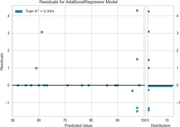
Boosted GPR Residuals.
In order to provide more in-depth information about the effect of different operational factors on the POME production yield, the study of 3D diagrams can be very effective. Therefore, the 3D graphs in Figs. 9-14 were obtained from the Boosted GPR model to show the effect of different operational parameters on the yield of fatty acid methyl ester production from Papaya oil. In each 3D diagram, the dual effect of factors on the fuel production yield was examined while the other two parameters remained constant. Figs. 9-11 show the expected results of POME (Y) yield vs. reaction temperature for various parameters such as catalyst dose, treatment period, and methanol to Papaya oil molar ratio, respectively. As can be seen by raising the temperature of the reaction (X1) the yield of fuel preparation increases however increasing the reaction temperature more than about 62.5 °C lead to rapid decrease in the POME. This fact is obvious in Fig. 9 and there should be an optimum value for temperature of the reaction. A similar pattern was found when the amount of catalysts was increased (X2). By rising the catalysts mass, the fuel preparation yield (Y) is also increased but as can be seen higher amount of catalysts led to decrement in the production yield (Sumayli and Alshahrani, 2023). Fig. 10 illustrates the effect of reaction temperature on the efficiency of POME production by changing the time of process between 0.5 and 10.5 min, while the catalysts amount and methanol to oil molar ratio were kept constant. Based on obtained results in this figure, increasing the reaction time to roughly 6.0 min enhanced the reaction yield, however the exact amount of optimum time of reaction should be obtained. When the reaction temperature is elevated from 50 ⁰C to 60 ⁰C, there is a possibility for an increase in POME yield. This may occur as a result of the rapid dipole rotation generating heat (Hong et al., 2016). Higher increment in the reaction temperature had a reverse effect of the POME production yield, therefore, the optimum amount of temperature should be obtained to achieve the maximum production of biodiesel. The impact of the molar ratio of methanol to papaya oil (X4) and the reaction temperature on POME production yield is demonstrated in Fig. 11. The results indicate that lower values of temperature and molar ratio of methanol to papaya oil resulted in lower POME production yield. By raising the molar ratio, the yield of POME production was increased significantly, and the optimum value for highest POME production yield should be determined. On the other hand, in temperatures more than 70 ⁰C the POME production yields were reduced which can be due to the vaporization of methanol in the reaction media (Nayak and Vyas, 2019).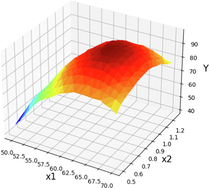
The prediction surface displayed alongside the X1 and X2 projections in optimized Boosted GPR model. X3 = 5.5 and X4 = 12. The optimal value is 98.87 for X1 = 63 and X2 = 0.814.
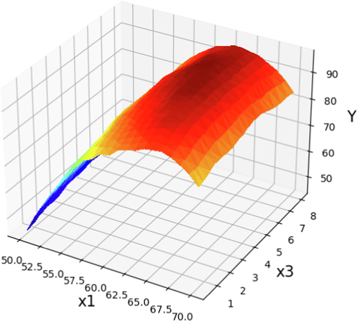
The prediction surface displayed alongside the X1 and X3 in optimized Boosted GPR model. X2 = 1 and X4 = 12. Optimal value is 97.11 for X1 = 63 and X3 = 5.77.
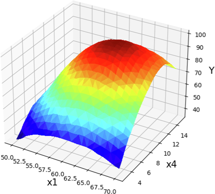
The prediction surface displayed alongside the X1 and X4 in optimized Boosted GPR model. X2 = 1 and X3 = 5.5. Optimal value is 98.93 for X1 = 62 and X4 = 9.46.
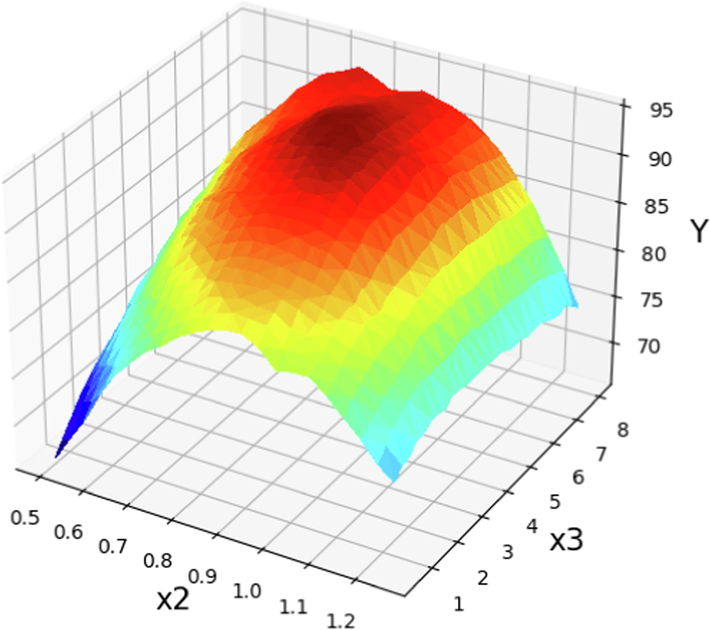
The prediction surface displayed alongside the X2 and X3 in optimized Boosted GPR model. X1 = 60 and X4 = 12. Optimal value is 95.05 for X2 = 0.892 and X3 = 4.66.
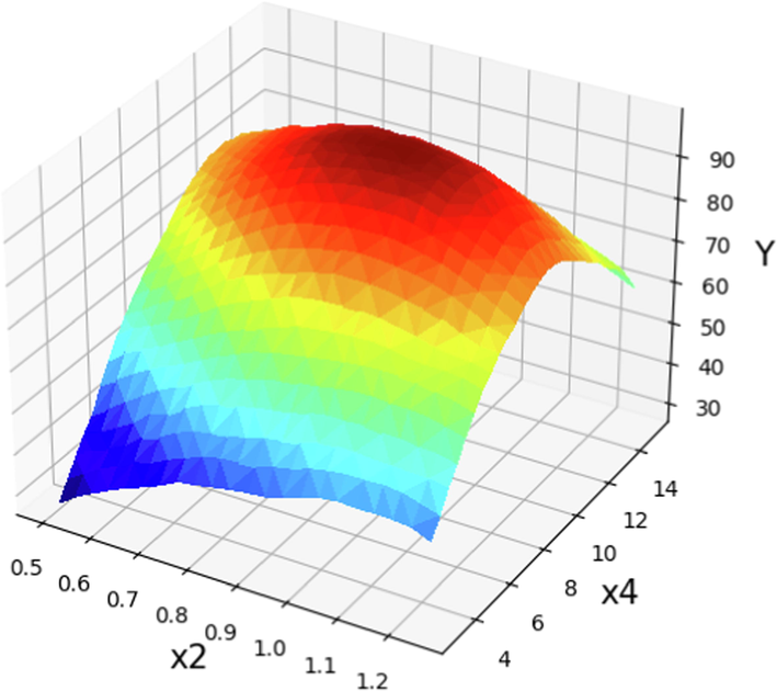
The prediction surface displayed alongside the X2 and X4 in optimized Boosted GPR model. X1 = 60 and X3 = 5.5. Optimal value is 99.63 for X2 = 0.928 and X4 = 9.92.
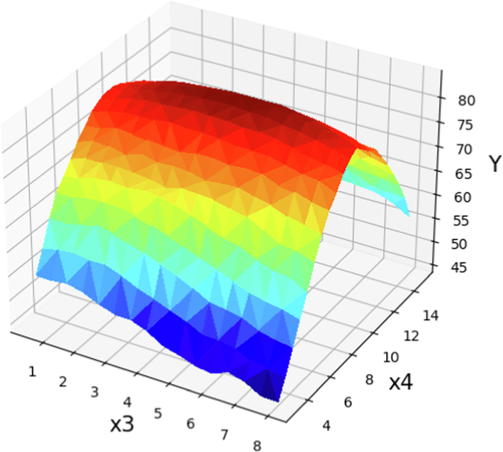
The prediction surface displayed alongside the X3 and X4 in optimized Boosted GPR model. X1 = 60 and X2 = 1.25. Optimal value is 84.6 for X3 = 4.5 and X4 = 9.6.
In order to evaluate the effect of catalyst amount on the POME production yield, the 3D plots of catalyst amount versus reaction time (min) and methanol to Papaya oil molar ration were studied. The obtained results are depicted in Figs. 12 and 13. As can be inferred from Fig. 12 while the two other parameters remained constant (X1 = 60 and X4 = 12), at low catalyst loading, increasing the time improved the interaction of triglycerides with methanol and increase the POME production yield. But by increasing the amount of catalyst had revers effect on the production yield which can be due to the uninvited soap formation of fatty acid which lead to entrainment of biodiesel (Dharma et al., 2016). Fig. 14 depicts the effect of catalyst concentration (X2, NaOH) and methanol to Papaya oil molar ratio (X4) on POME efficiency while two other parameters (reaction temperature and time) were kept constant (Sumayli and Alshahrani, 2023). Obviously, when the molar ratio and catalyst amount are very small, lower POME production yields were obtained which can be due to the fast consumption of methanol and catalyst during the reaction (Liu and Zhang, 2023). By increasing these amounts the POME production yields will increase however the production yield reach to a maximum and after that start to reduction. The reason for this could be attributed to the possibility of side reactions that result in the consumption of both the catalyst and methanol. As a consequence of the increased content of the catalyst and methanol, there is a decrease in POME efficiency.
Fig. 14 shows the dual effect of reaction time and methanol to Papaya oil molar ratio on the POME production yield while the temperature of reaction and amount of catalyst kept constant. Accordingly, lower POME efficiency (Y) is observed at low ratio of methanol to Papaya oil (X4) and short reaction time (X3). By increasing the time and molar ration the POME production yield was increased. As can be realized, increasing the molar ratio up to 10.3 resulted in a modest improvement in POME efficiency, but after that, POME production yield was declined. This could be attributed to the increased solubility of methanol in both phases, leading to greater difficulty in their separation (Liu and Zhang, 2023; Nayak and Vyas, 2019).
Figs. 15-18 depict the impact of each parameter on the POME production yield through 2D diagrams. Each diagram displays the effect of one operating factor while keeping the other three constant. As illustrated in Fig. 15, an increase in the reaction media temperature resulted in an increase in POME yield. This can be explained by the reduction of oil viscosity and increase of the reaction rate. Also, the higher temperature can lead to higher solubility of oil in alcohol phase. The trend persisted until the temperature hit 62 °C, beyond which the POME production yield declined due to methanol vaporization, consistent with the 3D diagrams discussed earlier. Fig. 16 displays the individual effect of catalysts amount on the yield of POME production in the transesterification process. Increasing the amount of catalyst leads to improvement in production yield which is due to higher formation of methoxy radicals and more interaction with triglyceride which produces the final product as biofuel. However, as can be seen in this figure, a higher amount of catalyst had the revers effect and reduced the POME production yield. As mentioned before, a higher amount of catalyst lead to side reactions which are undesired.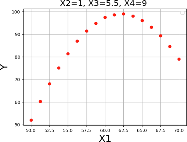
Trends for X1 on the POME production yield.
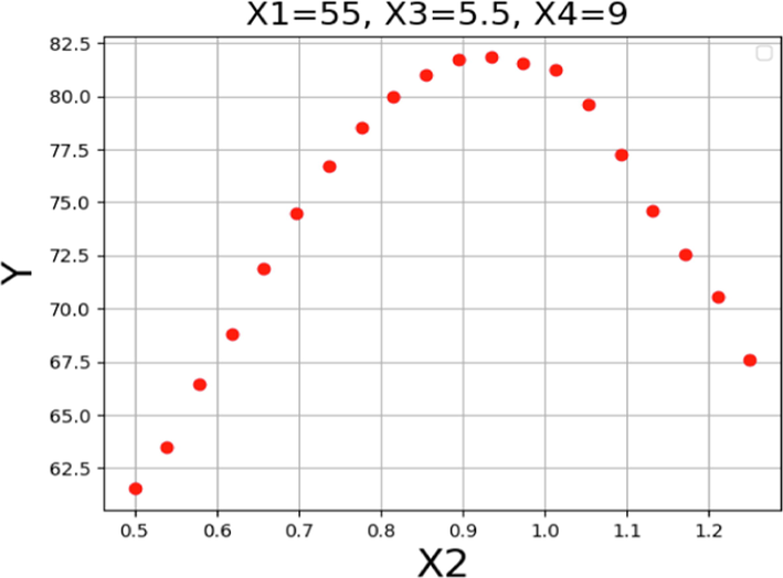
Trends for X2 on the POME production yield.
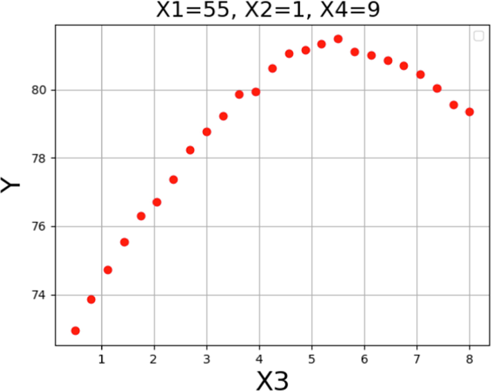
Trends for X3 on the POME production yield.
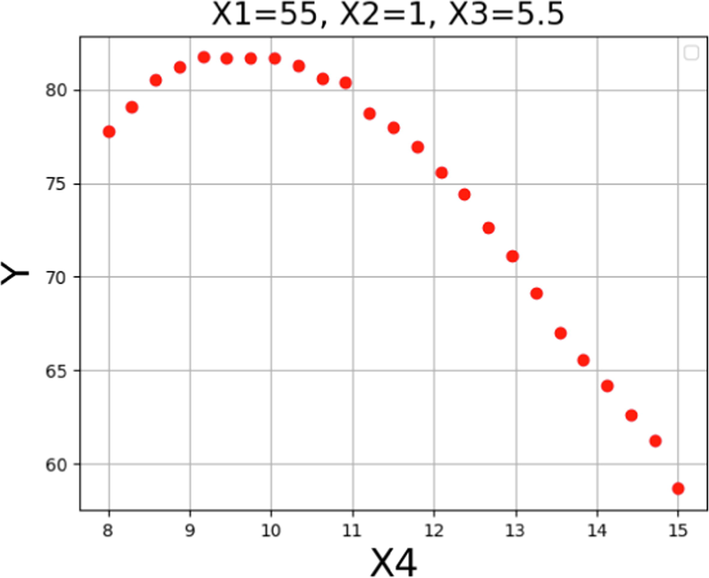
Trends for X4 on the POME production yield.
The individual effect of time and the molar ration of methanol to Papaya oil on the process efficiency are presented in Figs. 17 and 18, respectively. Based on the results, it can be said that by increasing the molar the ratio up to around 10 the POME yield was increased but higher value of methanol to Papaya oil reduced the process efficiency. The reason can be explained by dilution of the amount of catalyst due to higher amount of methanol which reduces the reaction rate and POME production yield.
The optimal values of operating parameters molar ratio play an important role in improvement of the POME production yield. Therefore, in this study the optimization of the POME production yield was performed by applying the final boosted GPR model to the range of accessible data. The best output values and the matching inputs are displayed in Table 3. It is clear that the maximum POME production yield of 99.89% was attained under with optimized condition of temperature of 62.5 ⁰C, catalyst amount of 0.8125 wt%, reaction time of 6.469 min, and methanol to oil molar ratio of 10.33.
X1
X2
X3
X4
Y
62.5
0.8125
6.469
10.33
99.89
5 Conclusion
In this research, ML methods were employed to successfully model the biodiesel production process from Papaya oil through the transesterification reaction. In machine learning problems, model selection is extremely crucial. The approaches employed in this study were chosen after a thorough examination and preliminary analysis of various current regression models. To predict the production of Papaya oil methyl ester, the multilayer perceptron (MLP), Gaussian Process Regression (GPR), and K-nearest neighbor (KNN) regression models were used, also adaptive boosting was applied for amplification. To produce the final models with ideal configurations, the basic hyperparameters of all selected models were modified depending on accuracy and generality. The catalyst amount, methanol to Papaya oil molar ratio, reaction temperature, and time were considered as input features of models while the POME production yield were set as the model output. The higher value of R2-scores (0.993) together with the lowest values of RMSE (4.8150) and MAE (2.3184) values for Boosted GPR model suggested that could predict the experimental results with high accuracy. The obtained results showed that all the studied operating parameters had a key effect on POME production yield. Optimization of these biodiesel production process, suggested that within the range of the given operating parameters, the ideal temperature, catalyst amount, duration, and methanol to oil molar ratio were 62.5 °C, 0.8125 wt%, 6.47 min, and 10.33, respectively, with an output of 99.89. Overall, the proposed ML strategy can be performed for prediction, modeling, and optimization of production of different biodiesel.
Declaration of Competing Interest
The authors declare that they have no known competing financial interests or personal relationships that could have appeared to influence the work reported in this paper.
References
- Machine learning technology in biodiesel research: a review. Prog. Energy Combust. Sci.. 2021;85:100904
- [Google Scholar]
- Methanolysis of Carica papaya seed oil for production of biodiesel. J. Fuels. 2014;2014
- [Google Scholar]
- Bishop, C.M. and N.M. Nasrabadi, Pattern recognition and machine learning. Vol. 4. 2006: Springer.
- Comparison of model selection for regression. Neural Comput.. 2003;15(7):1691-1714.
- [Google Scholar]
- Solid heterogeneous catalysts for production of biodiesel from trans-esterification of triglycerides with methanol: a review. Acta Chim. Pharma. Ind.. 2012;2(1):8-14.
- [Google Scholar]
- Gaussian process modelling with Gaussian mixture likelihood. J. Process Control. 2019;81:209-220.
- [Google Scholar]
- Mean absolute percentage error for regression models. Neurocomputing. 2016;192:38-48.
- [Google Scholar]
- Greenhouse gas emissions, non-renewable energy consumption, and output in South America: the role of the productive structure. Environ. Sci. Pollut. Res. 2020:1-15.
- [Google Scholar]
- Optimization of biodiesel production process for mixed Jatropha curcas–Ceiba pentandra biodiesel using response surface methodology. Energ. Conver. Manage.. 2016;115:178-190.
- [Google Scholar]
- Greedy function approximation: a gradient boosting machine. Ann. Stat. 2001:1189-1232.
- [Google Scholar]
- Papaya (Carica papaya L.): Origin, domestication, and production. In: Genetics and genomics of papaya. Springer; 2014. p. :3-15.
- [Google Scholar]
- Transesterification of rapeseed oil for the production of biodiesel using homogeneous and heterogeneous catalysis. Fuel Process. Technol.. 2009;90(7–8):1016-1022.
- [Google Scholar]
- Stream water temperature prediction based on Gaussian process regression. Expert Syst. Appl.. 2013;40(18):7407-7414.
- [Google Scholar]
- Theory of the backpropagation neural network. In: Neural networks for perception. Elsevier; 1992. p. :65-93.
- [Google Scholar]
- Preparation of waste cooking oil based biodiesel using microwave irradiation energy. J. Ind. Eng. Chem.. 2016;42:107-112.
- [Google Scholar]
- All pixels calibration for ToF camera. IOP Conf. Ser.: Earth Environ. Sci.. 2018;170(2):022164
- [Google Scholar]
- The threat to climate change mitigation posed by the abundance of fossil fuels. Clim. Pol.. 2019;19(2):258-274.
- [Google Scholar]
- Development of multiple machine-learning computational techniques for optimization of heterogenous catalytic biodiesel production from waste vegetable oil. Arab. J. Chem.. 2022;15(6):103843
- [Google Scholar]
- Improving biodiesel fuel properties by modifying fatty ester composition. Energ. Environ. Sci.. 2009;2(7):759-766.
- [Google Scholar]
- Transesterification of neat and used frying oil: optimization for biodiesel production. Fuel Process. Technol.. 2006;87(10):883-890.
- [Google Scholar]
- Transesterification catalyzed by ionic liquids on superhydrophobic mesoporous polymers: heterogeneous catalysts that are faster than homogeneous catalysts. J. Am. Chem. Soc.. 2012;134(41):16948-16950.
- [Google Scholar]
- Optimization of biodiesel production from oil using a novel green catalyst via development of a predictive model. Arab. J. Chem.. 2023;16(6):104785
- [Google Scholar]
- The production of prediction: What does machine learning want? Eur. J. Cult. Stud.. 2015;18(4–5):429-445.
- [Google Scholar]
- Evaluation of four supervised learning methods for groundwater spring potential mapping in Khalkhal region (Iran) using GIS-based features. Hydrgeol. J.. 2017;25(1):169-189.
- [Google Scholar]
- Optimization of microwave-assisted biodiesel production from Papaya oil using response surface methodology. Renew. Energy. 2019;138:18-28.
- [Google Scholar]
- Multilayer perceptron tutorial. School of Computing: Staffordshire University; 2005.
- Pardal, A.C., et al., Transesterification of rapeseed oil with methanol in the presence of various co-solvents. 2010.
- Oak wood ash/GO/Fe3O4 adsorption efficiencies for cadmium and lead removal from aqueous solution: Kinetics, equilibrium and thermodynamic evaluation. Arab. J. Chem.. 2021;14(3):102991
- [Google Scholar]
- A quantitative study of experimental evaluations of neural network learning algorithms: current research practice. Neural Netw.. 1996;9(3):457-462.
- [Google Scholar]
- Predicting cetane number, kinematic viscosity, density and higher heating value of biodiesel from its fatty acid methyl ester composition. Fuel. 2012;91(1):102-111.
- [Google Scholar]
- Gaussian processes in machine learning. In: Summer school on machine learning. Springer; 2003.
- [Google Scholar]
- The use and misuse of statistics in space physics. J. Geomag. Geoelec.. 1990;42(9):1145-1174.
- [Google Scholar]
- Prediction of density and viscosity of biofuel compounds using machine learning methods. Energy Fuel. 2012;26(4):2416-2426.
- [Google Scholar]
- Senders, J.T., et al., Machine learning and neurosurgical outcome prediction: a systematic review. World neurosurgery, 2018. 109: p. 476-486. e1
- Alternatives to the global warming potential for comparing climate impacts of emissions of greenhouse gases. Clim. Change. 2005;68(3):281-302.
- [Google Scholar]
- Biodiesel development from rice bran oil: transesterification process optimization and fuel characterization. Energ. Conver. Manage.. 2008;49(5):1248-1257.
- [Google Scholar]
- Comparison of multilayer perceptron and radial basis function in predicting success of new product development. Eng. Technol. Appl. Sci. Res. 2017:7.
- [Google Scholar]
- A Comparative Study of Classification and Regression Algorithms for Modelling Students' Academic Performance. International Educational Data Mining Society; 2015.
- Modeling and prediction of biodiesel production by using different artificial intelligence methods: Multi-layer perceptron (MLP), Gradient boosting (GB), and Gaussian process regression (GPR) Arab. J. Chem.. 2023;16(7):104801
- [Google Scholar]
- Activity of homogeneous and heterogeneous catalysts, spectroscopic and chromatographic characterization of biodiesel: a review. Renew. Sustain. Energy Rev.. 2012;16(8):6303-6316.
- [Google Scholar]
- Wang, H., Y. Guan, and B. Reich. Nearest-neighbor neural networks for geostatistics. in 2019 International Conference on Data Mining Workshops (ICDMW). 2019. IEEE.
- A review of machine learning for the optimization of production processes. Int. J. Adv. Manuf. Technol.. 2019;104(5):1889-1902.
- [Google Scholar]
- Yang, J., et al. Computation of two-layer perceptron networks’ sensitivity to input perturbation. in 2008 International Conference on Machine Learning and Cybernetics. 2008. IEEE.
- Identifying degradation patterns of lithium ion batteries from impedance spectroscopy using machine learning. Nat. Commun.. 2020;11(1):1-6.
- [Google Scholar]
- Feature extraction and physical interpretation of melt pressure during injection molding process. J. Mater. Process. Technol.. 2018;261:50-60.
- [Google Scholar]


