Hybrid mechanistic approach in the estimation of flow properties in cylindrical membrane modules

Fang Peng; Wei Yang; Yi Liu

doi:10.1016/j.arabjc.2022.104306

View/Download PDF

Buy Reprints

PDF

Translate this page into:

Original article

12 2022

:15;

104306

doi:

10.1016/j.arabjc.2022.104306

Hybrid mechanistic approach in the estimation of flow properties in cylindrical membrane modules

Fang Peng^{^a,⁎}, Wei Yang^{^a}, Yi Liu^{^b}

a Department of Mechanical and Electrical Engineering, Inner Mongolia Vocational College of Chemical Engineering, Hohhot, Inner Mongolia 010000, China

b Hangzhou Xinya Low Temperature Technology Co., Ltd, Hangzhou, Zhejiang 310000, China

⁎Corresponding author. pfyouxiang82@126.com (Fang Peng)

Received: 2022-2-26, Accepted: 2022-9-24,

Disclaimer:
This article was originally published by Elsevier and was migrated to Scientific Scholar after the change of Publisher.

Peer review under responsibility of King Saud University.

Abstract

A hybrid computational approach was employed for simulation of molecular separation using polymeric membranes. The considered system is a cylindrical membrane module in which the mass transfer equations were solved numerically using CFD (Computational Fluid Dynamics) to obtain the concentration of the species, and then the simulation results were used in machine learning models. Indeed, the CFD simulation results were used as the inputs for several machine learning models to obtain the hybrid model. We have a dataset with more than 2000 data points and two input features (r and z). Also, the only output is C which is the concentration of the species in the feed channel of membrane module. KNN (K nearest neighbor), PLSR (Partial Least Square Regression), and SGD (Stochastic Gradient Descent) are the models employed in this research to analyze the mentioned data set. Models were optimized with their hyper-parameters and finally evaluated with different statistical metrics. MAE error metric is 3.4, 5.1, and 5.5 for KNN, SGD, and PLSR. Also, they have 0.998, 0.997, 0.896 coefficient of determination (R²) respectively. Finally, based on the overall results, KNN with K = 8 is selected as the best model in this study for simulation of the membrane system. The final maximum error is also 1.35E+02.

Keywords

CFD

Computational simulation

Fluid flow

Separation

Machine learning

Environmental

Show Related Articles from PubMed

1 Introduction

Separation and removal of water pollutants is a great subject of interest which can be done using molecular separation methods via different separation techniques. From the environmental perspective, pollutant molecules must be removed from effluents prior to discharge to the environment, as they might cause severe health problems (Fan et al., 2022; Ge et al., 2019; Guan et al., 2021; Liu et al., 2020, 2022; Bai et al., 2021 ). The process of molecular separation has also wide applications in different fields such as nanotechnology-based areas, biochemical, pharmaceuticals, food, etc. (Wang et al., 2022a, 2022b; Xu et al., 2022; Yang et al., 2021; Yu et al., 2022a, 2022b ). The selection and design of appropriate method is of fundamental importance to achieve the best and optimum conditions for the separation yield (Wang et al., 2022c, 2021; Zhang et al., 2022 ).

The molecular separation based on membrane technology offers superior advantages in process engineering field which makes this novel process efficient for separation and removal of target molecules from a mixture (Han et al., 2022; Chen and Yang, 2022; Wang et al., 2022d ). The main advantage of membrane processes in molecular separation is that these processes can be regarded as green technology for separation, as no organic solvent is required in most of the membrane processes. In some cases, organic solvents are used for the separation such as those in membrane contactors for CO₂ capture and liquid extraction (Sabzekar et al., 2022; Petukhov et al., 2022; Liu et al., 2022 ).

To design and optimize the membrane separation process for a given target molecule, computational simulation can be employed in this regard to improve the separation process (Mou et al., 2022; Liu et al., 2022). The membrane-based computational simulation can be performed mainly using either computational fluid dynamics (CFD) or machine learning models. CFD methods are considered to be mechanistic models which provide process understanding, while the machine learning (ML) models are black-box models and use dataset for training algorithms. Integration of both models would be a novel idea in molecular separation which is the main focus of the current research.

A growing number of scientific disciplines are transitioning to machine learning (ML) methodologies that are progressively taking on the roles of classical computing methods. These techniques can be applied to solve problems in a number of ways. There is some correlation between inputs and outputs derived from these models, which produce some predictions (Alpaydin, 2020; Bishop, 2006; Carbonell et al., 1983 ).

KNN (K nearest neighbor) is one of the models that have been selected for this study to model the molecular separation case study. As well as being used for classification problems, it can also be used for regression problems. The application of this method is, however, more widely used in the field of classification problems. As the name implies, The K nearest neighbor algorithm is a simple algorithm that stores all of the available cases. New cases are estimated by the K closest neighbors based on their majority votes or average. In a distance function, the case being assigned to a class will be the one that has the highest frequency among its K nearest neighbors (Song et al., 2017; Kohli et al., 2021).

In this study, partial least square regression is also used as one of the models. In many problems, the partial least square regression (PLSR) model is a method that combines spectral measurements and chemical composition or physical properties of solids and charred materials to produce a rapid multivariate analysis with several variables (Xie and Chen, 2022; Boulesteix and Strimmer, 2007).

It is also relevant to note that Stochastic Gradient Descent (SGD) is a straightforward and effective technique for classifying and regressing linear data with convex loss functions, such as Support Vector Machines (linear) and Logistic Regression (linear). In the field of machine learning, the idea of SGD has been around for a long time; however, it is only relatively recently that it has received a significant amount of attention in the context of large-scale learning (Ighalo et al., 2020; Bottou, 1998).

In the current research, we have employed for the first time, the three mentioned machine learning methods for integration with CFD simulation to build hybrid modeling for simulation of a molecular separation case study via polymeric membrane technique.

2 Methodology

2.1

2.1 CFD method of modeling

As stated before, we used CFD simulation results in modeling of membrane separation process using machine learning models. In the first step of this work, CFD was performed to simulate removal of a species using polymeric cylindrical shape membrane. A simple geometry was designed and the mass transfer equations including convection and diffusion was solved for the feed, membrane, and permeate channels of the membrane module (Shirazian et al., 2012). Cylindrical coordinate was used for deriving and solving the governing equations. The main mass transfer equation can be expressed as (Rezakazemi et al., 2019):

(1)

D_{AB} [\frac{\partial^{2} C}{{\partial r}^{2}} + \frac{1}{r} \frac{\partial C}{\partial r} + \frac{\partial^{2} C}{{\partial z}^{2}}] = V \frac{\partial C}{\partial z}

where D_AB refers to the diffusion coefficient and C refers to the species concentration. Also, r and z refer to the radial and axial coordinate, while V is the velocity vector. Finite element method was used to solve Eq. (1) numerically (Rezakazemi et al., 2019).

2.2

2.2 Partial least squares regression (PLSR)

We have used a number of machine learning models to integrate to the CFD results for simulation of the membrane process in which PLSR is the first model which is utilized in this research. Using the covariance matrix, partial least squares regression is an efficient, quick and optimal regression technique. Partial Least Squares Regression, or PLS Regression, is the most common Partial Least Squares model. All other models in the family of PLS models are based on partial least squares regression. Regression models are applicable when you have numerical dependent variables (Bjørn-Helge et al., 2019). In the field of engineering and science, PLSR acts as a bilinear factor model which is extensively used in a variety of engineering and science fields. As a result, it performs well on matrices X that contain many noisy and collinear factors. According to the following Equations, the PLSR should have an optimal factor number (Abdi, 2010; Guo et al., 2021):

(2)

S_{S S, h} = \sum_{i = 1}^{n} {(y_{i} - {\hat{y}}_{h i})}^{2}

(3)

S_{P R E S S, h} = \sum_{i = 1}^{n} {(y_{i} - {\hat{y}}_{h (- i)})}^{2}

(4)

{Q_{h}}^{2} = 1 - \frac{S_{P R E S S, h}}{S_{S S, h}}

where

y_{i}

is the original data and

{\hat{y}}_{hi}

is the fitted value of the i-th data point calculated from all data points and the h component of the regression model. By removing I as a data point from the modeling process and extracting the h component from the resulting regression model, we get the

{\hat{y}}_{h (- i)}

notation, which indicates that

y_{i}

was determined using the latter. In the presence of

{Q_{h}}^{2} \geq 0.0975

, the addition of a new component greatly enhances the predictive power of the constructed model; in the other cases, the added new component has no meaningful significance (Guo et al., 2021; Elden, 2004).

2.3

2.3 KNN method

This model is a straightforward classification or regression model that uses the k-Nearest Neighbor estimation technique as an instance-based machine learning model. A second reason why this is an inefficient technique is that it does not generalize from the subset of data used for training. This means that when testing and for unknown data, the full training subset is retained in addition to the testing subset. In KNN regression, the test examples are identified by comparing them to the training examples, in order to learn the regression model (Cover, 1968).

Suppose $T = [(x_{1}, y_{1}), \dots, (x_{N}, y_{N})]$ indicate distance parameterized training data and d, $x_{i} = (x_{i 1}, \dots, x_{im})$ is a representation of the i-th instance based on m input variables together with corresponding target output y_i. The number N represents the quantity of examples that have been provided. The d_i must be calculated between a test data point (x) and all other points x_i ∈ T. Then sort the d_i distances for a test data point x. If d_i is ranked as the i^th position, the d_i matching sample is referred to as the i^th nearest neighbor NNi(x), and its target is denoted by y_i (x). Lastly, $\hat{y}$ denotes the average of the regression outputs of KNN to x, i.e., $\hat{y} = \frac{1}{k} \sum_{i = 1}^{k} y_{i} (x)$ . Following are the steps involved in the KNN regression algorithm (Song, 2017):

Inputs: training samples $\{x_{i}, y_{i}\}, x_{i}$ : input features, $y_{i}$ : output value, a single test data point x
Algorithm:
- Compare each x_i with the query data point(x) and calculate the distance between them.
- Search for $k$ closet data points $x_{i 1} \dots x_{ik}$ and their target outputs $y_{i 1} \dots y_{ik}$
- output:

\hat{y} = \frac{1}{K} \sum_{j = 1}^{k} y_{i_{j}}

2.4

2.4 Stochastic Gradient Descent (SGD)

SGD estimates the objective function gradient using a subset of training samples and dynamically adjusts the parameters. Batch size refers to the number of training samples employed. In the case of larger batches, the SGD simply changes into a gradient descent when the batch size increases. Although this is a very slow solution to convergence, it can be sped up by changing parameters more often with a small batch size (Haider et al., 2021).

The stochastic gradient descent (SGD) method is an algorithmic simplification of GD that uses only a sample from the dataset to estimate the gradient on each update iteration:

(5)

w_{t + 1} = w_{t} - γ_{t} \nabla_{w} Q (z_{i}, w_{t})

Under sufficient regularity conditions, it usually achieves a fast convergence when the learning rate is $γ t^{- 1}$ .

Each time the SGD iterates, it picks random samples from a finite training set. Most training sets have a bigger number of iterations than the number of training iterations. In this way, most of the data points in the training subset can be traversed by the average traversal of the data. Additionally, some of them will be run multiple times so that the expected risk can be directly optimized (Johnson and Zhang, 2013).

3 Results and discussions

3.1

3.1 CFD results

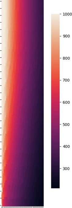
As explained earlier, we have performed CFD simulations for removal of species using a cylindrical membrane module. At the beginning of this work, the concentration distribution of the species was calculated using the CFD which uses finite element method. The results of the concentration (C) distribution are illustrated in Fig. 1 as 2D plot in cylindrical coordinate. The feed enters the membrane module from the bottom where the concentration is the highest (∼1000) and leaves the module from the top side where the concentration decreases due to the mass transfer of species towards the polymeric membrane surface. It should be noted that we presented only the feed channel of the membrane module, and the membrane itself, and the permeate side is not represented in Fig. 1. Also, we used the feed channel data for training and validation of the machine learning models.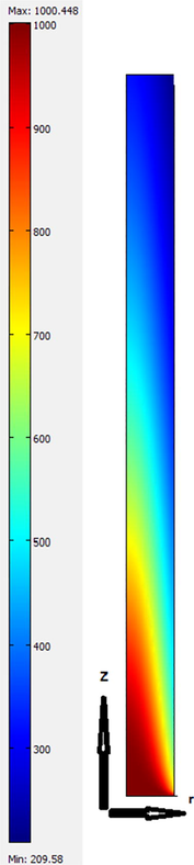

Concentration (C) distribution of species in the feed channel of membrane calculated using CFD method.

3.2

3.2 Machine learning results

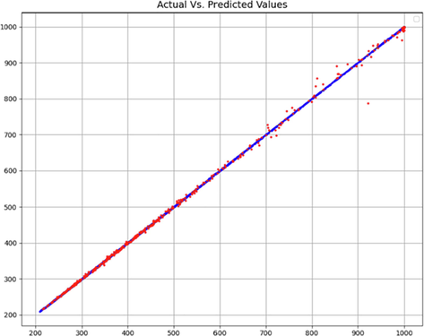
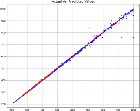
In order to obtain a suitable evaluation, the selection of the ratio of training and testing in the data is of particular importance. For this purpose, we tested this work with different values and evaluated the accuracy of the models (on average) in order to choose this configuration accurately. In Fig. 2, the effect of the ratio of the data of the train and the test on the accuracy of the model is examined, and according to this figure, 90% of the data is considered as the train and 10% as the test. Figs. 3 and 4 also show the comparison of the most 50% and 90% data in terms of the proximity of the expected and predicted data, which confirms the above fact.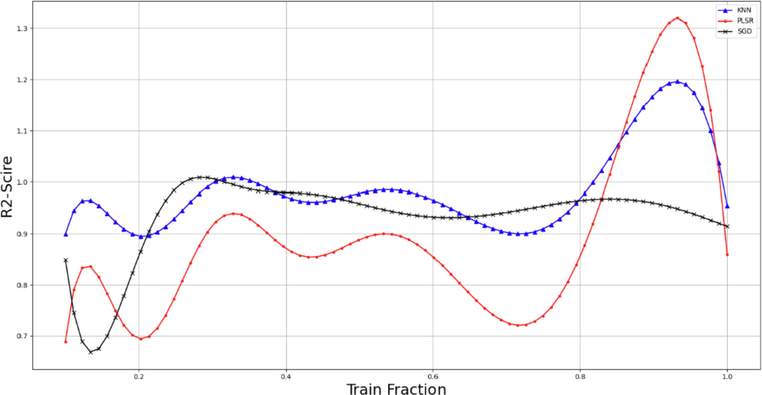

Impact of different train fractions on model accuracy.

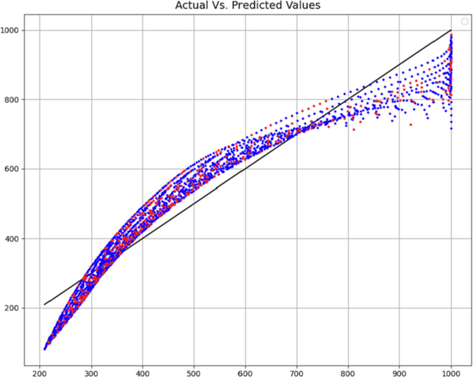
0.5 training set – Comparison of predicted and actual C values.

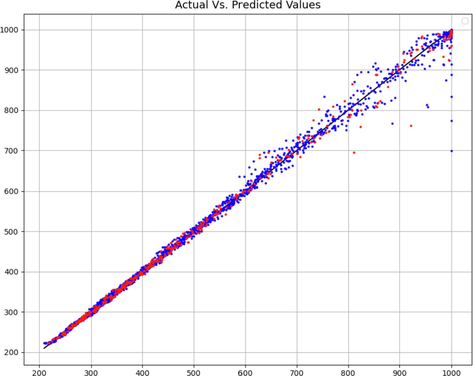
0.9 training set – Comparison of predicted and actual C values.

For the purpose of comparing and analyzing final results, three models' parameters are optimized, and final models are implemented based on these configurations. For example, in Fig. 5, as an example of the hyper-parameter optimization result, the value of K (number of neighbors) in the KNN is shown for different values, for which the value of 8 was finally selected.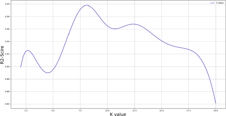

Impact of value of K in KNN model on performance of model.

In regression modeling, a model error represents a deviation of the dataset from a reference set. A regression line is defined as the line that is closest to the observable data points. If there are multiple data points, the model's error is estimated using the below parameters (Hu et al., 2022):

MAE: A mean is found by averaging the absolute values of the errors (Willmott and Matsuura, 2005; Botchkarev, 2018):

(6)

MAE = \frac{\sum_{i = 1}^{n} | y_{i} - x_{i} |}{n}

RMSE: The root mean square error is one of the most commonly used model performance evaluation statistics which is expressed as (Willmott and Matsuura, 2005):

(7)

RMSE = \sqrt{\frac{\sum_{i = 1}^{n} {(x_{i} - y_{i})}^{2}}{n}}

R²-Score

As can be seen from Table 1, the numerical results of the introduced models can be compared with each other. We can clearly see from the table that the KNN model is the most accurate model. This is because it has the most accurate results in terms of all the metrics, thus making it the most general model. There is also a confirmation of this issue in the validation Figs. 6–8 .

Table 1 The model results and their comparisons.

Models	MAE	RMSE	Max Error	R²
KNN	3.43514E+00	8.7266E+00	1.34717E+02	0.9983
SGD	5.13564E+00	1.1170E+01	1.64051E+02	0.9973
PLSR	5.51127E+01	6.5923E+01	1.97509E+02	0.8969

KNN model – Comparison of predicted and actual C values.

SGD model – Comparison of predicted and actual C values.

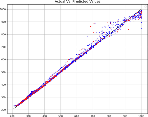
PLSR model – Comparison of predicted and actual C values.

The plot of prediction surface in the final model is shown in Fig. 9 for the best model which is KNN. Also, this diagram is similarly shown for two other models that are not the best case in Figs. 10 and 11. It is clearly seen that the developed machine learning models are capable of capturing the variations of the species concentration in the membrane feed channel with great accuracy.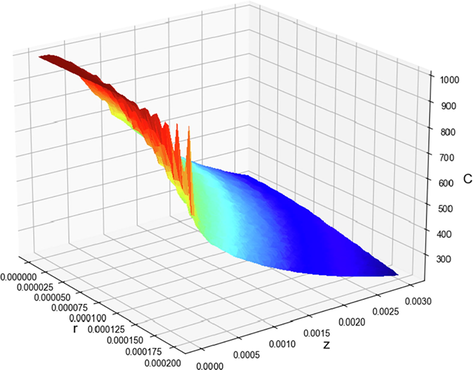

Final KNN model. 3D projection of output with model.

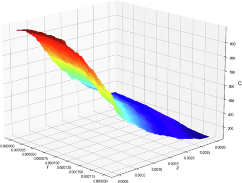
Final SGD model. 3D projection of output with model.

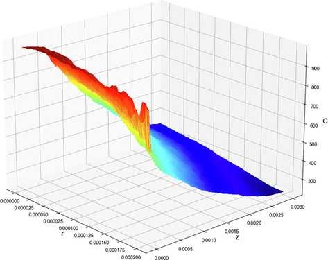
Final PLSR model. 3D projection of output with model.

In order to have a better view of the result of the final model, two heat map diagrams are shown in color in Figs. 12 and 13, in which the inputs are scaled in the first and not in the second illustration. Having looked at the results, it is concluded that the machine learning models can predict the CFD simulation results with acceptable accuracy and thereby can minimize the computational expenses for CFD simulation of large-scale systems which require high computational expenses.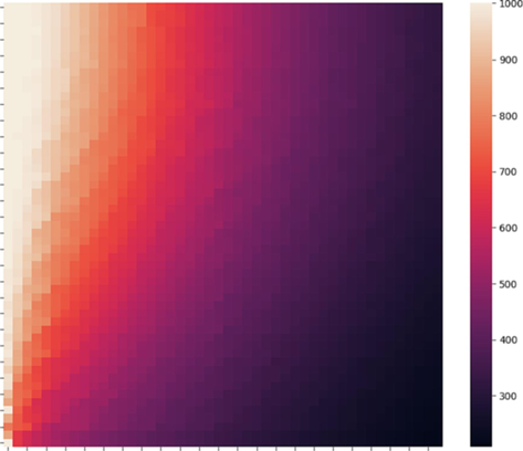

The heat map plot of final model. X-ax is r and Y-ax is z.

The unscaled heat map plot of final model. X-ax is r and Y-ax is z.

4 Conclusion

In this investigation, we have a dataset that contains over 2,000 individual data points and two distinct input features (r and z) which have been obtained from a CFD simulation of membrane system. Additionally, the only output is the concentration distribution of the species in the feed channel, i.e., C. KNN, which stands for “K nearest neighbor,” PLSR, which stands for “Partial Least Square Regression,” and SGD, which stands for “Stochastic Gradient Descent,” are the models that were used in this research to analyze the data set that was extracted from the CFD simulation of membrane. Following the optimization of the models with their hyper-parameters, the models were finally evaluated using a variety of statistical metrics. The MAE error metric for KNN, SGD, and PLSR are respectively 3.4, 5.1, and 5.5. In addition to this, the coefficient of determination (R²) for each of them is respectively 0.998, 0.997, and 0.896. In conclusion, the KNN model with a K value of 8 was chosen for process analysis, because it provided the best results across the board in this investigation. The maximum error possible in the final analysis is also 1.35E+02.

Acknowledgements

Study on the pulsation characteristics of non-stable pressure of centrifugal pumps (No. NJZY17450) is acknowledged.

Declaration of Competing Interest

The authors declare that they have no known competing financial interests or personal relationships that could have appeared to influence the work reported in this paper.

References

Abdi H., . Partial least squares regression and projection on latent structure regression (PLS Regression) Wiley Interdiscip. Rev.: Comput. Stat.. 2010;2(1):97-106.
[Google Scholar]
Alpaydin E., . Introduction to Machine Learning. MIT Press; 2020.
Bai B., . Cotransport of heavy metals and SiO2 particles at different temperatures by seepage. J. Hydrol.. 2021;597:125771
[Google Scholar]
Bishop C.M., . Pattern Recognition. Mach. Learn.. 2006;128:9.
[Google Scholar]
Bjørn-Helge, M., Wehrens, R., Hovde Liland, K., 2019. pls: Partial least squares and principal component regression. R package version, p. 2.7-2.
Botchkarev, A., 2018. Evaluating performance of regression machine learning models using multiple error metrics in azure machine learning studio. Available at SSRN 3177507.
Bottou L., . Online learning and stochastic approximations. On-line Learn. Neural Netw.. 1998;17(9):142.
[Google Scholar]
Boulesteix A.-L., Strimmer K., . Partial least squares: a versatile tool for the analysis of high-dimensional genomic data. Briefings Bioinf.. 2007;8(1):32-44.
[Google Scholar]
Carbonell J.G., Michalski R.S., Mitchell T.M., . An overview of machine learning. Mach. Learn. 1983:3-23.
[Google Scholar]
Chen Y., Yang X., . Molecular simulation of layered GO membranes with amorphous structure for heavy metal ions separation. J. Membr. Sci.. 2022;660:120863
[Google Scholar]
Cover T., . Estimation by the nearest neighbor rule. IEEE Trans. Inf. Theory. 1968;14(1):50-55.
[Google Scholar]
Elden L., . Partial least-squares vs. Lanczos bidiagonalization—I: analysis of a projection method for multiple regression. Comput. Stat. Data Anal.. 2004;46(1):11-31.
[Google Scholar]
Fan S., . A novel water-free cleaning robot for dust removal from distributed photovoltaic (PV) in water-scarce areas. Sol. Energy. 2022;241:553-563.
[Google Scholar]
Ge D., . Insight into the enhanced sludge dewaterability by tannic acid conditioning and pH regulation. Sci. Total Environ.. 2019;679:298-306.
[Google Scholar]
Guan Q., . Ultrasonic power combined with seed materials for recovery of phosphorus from swine wastewater via struvite crystallization process. J. Environ. Manage.. 2021;293:112961
[Google Scholar]
Guo Y., . Prediction of rice yield in East China based on climate and agronomic traits data using artificial neural networks and partial least squares regression. Agronomy. 2021;11(2):282.
[Google Scholar]
Haider S.A., Sajid M., Iqbal S., . Forecasting hydrogen production potential in islamabad from solar energy using water electrolysis. Int. J. Hydrogen Energy. 2021;46(2):1671-1681.
[Google Scholar]
Han M.-C., . Single-Side Superhydrophobicity in Si3N4-Doped and SiO2-Treated Polypropylene Nonwoven Webs with Antibacterial Activity. Polymers. 2022;14(14):2952.
[Google Scholar]
Hu X., . Predictive modeling and computational machine learning simulation of adsorption separation using advanced nanocomposite materials. Arabian J. Chem.. 2022;15(9):104062
[Google Scholar]
Ighalo J.O., Adeniyi A.G., Marques G., . Application of linear regression algorithm and stochastic gradient descent in a machine-learning environment for predicting biomass higher heating value. Biofuels Bioprod. Biorefin.. 2020;14(6):1286-1295.
[Google Scholar]
Johnson R., Zhang T., . Accelerating stochastic gradient descent using predictive variance reduction. Adv. Neural Inf. Process. Syst.. 2013;26
[Google Scholar]
Kohli S., Godwin G.T., Urolagin S., . Sales prediction using linear and KNN regression. In: Advances in Machine Learning and Computational Intelligence. Springer; 2021. p. :321-329.
[Google Scholar]
Liu W., . Different Pathways for Cr(III) Oxidation: Implications for Cr(VI) Reoccurrence in Reduced Chromite Ore Processing Residue. Environ. Sci. Technol.. 2020;54(19):11971-11979.
[Google Scholar]
Liu Y., . Modeling insights into the role of support layer in the enhanced separation performance and stability of nanofiltration membrane. J. Membr. Sci.. 2022;658:120681
[Google Scholar]
Liu Y., . Novel method for high-performance simultaneous removal of NOx and SO2 by coupling yellow phosphorus emulsion with red mud. Chem. Eng. J.. 2022;428:131991
[Google Scholar]
Liu M., . Continuous separation and recovery of high viscosity oil from oil-in-water emulsion through nondispersive solvent extraction using hydrophobic nanofibrous poly(vinylidene fluoride) membrane. J. Membr. Sci.. 2022;660:120876
[Google Scholar]
Mou J., . An effective hybrid collaborative algorithm for energy-efficient distributed permutation flow-shop inverse scheduling. Future Generation Computer Systems. 2022;128:521-537.
[Google Scholar]
Petukhov D.I., . Nanoporous polypropylene membrane contactors for CO2 and H2S capture using alkali absorbents. Chem. Eng. Res. Des.. 2022;177:448-460.
[Google Scholar]
Rezakazemi M., Mosavi A., Shirazian S., . ANFIS pattern for molecular membranes separation optimization. J. Mol. Liq.. 2019;274:470-476.
[Google Scholar]
Sabzekar M., . Cyclic olefin polymer membrane as an emerging material for CO2 capture in gas-liquid membrane contactor. J. Environ. Chem. Eng.. 2022;10(3):107669
[Google Scholar]
Shirazian S., . Hydrodynamics and mass transfer simulation of wastewater treatment in membrane reactors. Desalination. 2012;286:290-295.
[Google Scholar]
Song Y., . An efficient instance selection algorithm for k nearest neighbor regression. Neurocomputing. 2017;251:26-34.
[Google Scholar]
Wang X., . Radium and nitrogen isotopes tracing fluxes and sources of submarine groundwater discharge driven nitrate in an urbanized coastal area. Sci. Total Environ.. 2021;763:144616
[Google Scholar]
Wang J., . Performance synergism of pervious pavement on stormwater management and urban heat island mitigation: A review of its benefits, key parameters, and co-benefits approach. Water Res.. 2022;221:118755
[Google Scholar]
Wang Y., . Mo-modified band structure and enhanced photocatalytic properties of tin oxide quantum dots for visible-light driven degradation of antibiotic contaminants. J. Environ. Chem. Eng.. 2022;10(1):107091
[Google Scholar]
Wang X., . Highly selective membrane for efficient separation of environmental determinands: Enhanced molecular imprinting in polydopamine-embedded porous sleeve. Chem. Eng. J.. 2022;449:137825
[Google Scholar]
Wang Z., . Experimental Investigation on Fracture Properties of HTPB Propellant with Circumferentially Notched Cylinder Sample. Propellants Explos. Pyrotech.. 2022;47(7):e202200046.
[Google Scholar]
Willmott C.J., Matsuura K., . Advantages of the mean absolute error (MAE) over the root mean square error (RMSE) in assessing average model performance. Clim. Res.. 2005;30(1):79-82.
[Google Scholar]
Xie Z., Chen X., . Subsampling for partial least-squares regression via an influence function. Knowl.-Based Syst.. 2022;245:108661
[Google Scholar]
Xu D., . Coupling of sponge fillers and two-zone clarifiers for granular sludge in an integrated oxidation ditch. Environ. Technol. Innovation. 2022;26:102264
[Google Scholar]
Yang Y., . Construction of a novel lanthanum carbonate-grafted ZSM-5 zeolite for effective highly selective phosphate removal from wastewater. Microporous Mesoporous Mater.. 2021;324:111289
[Google Scholar]
Yu C., . Ag3PO4-based photocatalysts and their application in organic-polluted wastewater treatment. Environ. Sci. Pollut. Res.. 2022;29(13):18423-18439.
[Google Scholar]
Yu F., . A redox-active perylene-anthraquinone donor-acceptor conjugated microporous polymer with an unusual electron delocalization channel for photocatalytic reduction of uranium (VI) in strongly acidic solution. Appl. Catal. B. 2022;314:121467
[Google Scholar]
Zhang T., . Improving the humification and phosphorus flow during swine manure composting: A trial for enhancing the beneficial applications of hazardous biowastes. J. Hazard. Mater.. 2022;425:127906
[Google Scholar]

Introduction

Methodology

CFD method of modeling
Partial least squares regression (PLSR)
KNN method
Stochastic Gradient Descent (SGD)

Results and discussions

CFD results
Machine learning results

Conclusion

Fulltext Views
17

PDF downloads
0

View/Download PDF
Download Citations

BibTeX
RIS

Show Sections

[1] Abdi H., . Partial least squares regression and projection on latent structure regression (PLS Regression) Wiley Interdiscip. Rev.: Comput. Stat.. 2010;2(1):97-106.
[Google Scholar]

[2] Alpaydin E., . Introduction to Machine Learning. MIT Press; 2020.

[3] Bai B., . Cotransport of heavy metals and SiO2 particles at different temperatures by seepage. J. Hydrol.. 2021;597:125771
[Google Scholar]

[4] Bishop C.M., . Pattern Recognition. Mach. Learn.. 2006;128:9.
[Google Scholar]

[5] Bjørn-Helge, M., Wehrens, R., Hovde Liland, K., 2019. pls: Partial least squares and principal component regression. R package version, p. 2.7-2.

[6] Botchkarev, A., 2018. Evaluating performance of regression machine learning models using multiple error metrics in azure machine learning studio. Available at SSRN 3177507.

[7] Bottou L., . Online learning and stochastic approximations. On-line Learn. Neural Netw.. 1998;17(9):142.
[Google Scholar]

[8] Boulesteix A.-L., Strimmer K., . Partial least squares: a versatile tool for the analysis of high-dimensional genomic data. Briefings Bioinf.. 2007;8(1):32-44.
[Google Scholar]

[9] Carbonell J.G., Michalski R.S., Mitchell T.M., . An overview of machine learning. Mach. Learn. 1983:3-23.
[Google Scholar]

[10] Chen Y., Yang X., . Molecular simulation of layered GO membranes with amorphous structure for heavy metal ions separation. J. Membr. Sci.. 2022;660:120863
[Google Scholar]

[11] Cover T., . Estimation by the nearest neighbor rule. IEEE Trans. Inf. Theory. 1968;14(1):50-55.
[Google Scholar]

[12] Elden L., . Partial least-squares vs. Lanczos bidiagonalization—I: analysis of a projection method for multiple regression. Comput. Stat. Data Anal.. 2004;46(1):11-31.
[Google Scholar]

[13] Fan S., . A novel water-free cleaning robot for dust removal from distributed photovoltaic (PV) in water-scarce areas. Sol. Energy. 2022;241:553-563.
[Google Scholar]

[14] Ge D., . Insight into the enhanced sludge dewaterability by tannic acid conditioning and pH regulation. Sci. Total Environ.. 2019;679:298-306.
[Google Scholar]

[15] Guan Q., . Ultrasonic power combined with seed materials for recovery of phosphorus from swine wastewater via struvite crystallization process. J. Environ. Manage.. 2021;293:112961
[Google Scholar]

[16] Guo Y., . Prediction of rice yield in East China based on climate and agronomic traits data using artificial neural networks and partial least squares regression. Agronomy. 2021;11(2):282.
[Google Scholar]

[17] Haider S.A., Sajid M., Iqbal S., . Forecasting hydrogen production potential in islamabad from solar energy using water electrolysis. Int. J. Hydrogen Energy. 2021;46(2):1671-1681.
[Google Scholar]

[18] Han M.-C., . Single-Side Superhydrophobicity in Si3N4-Doped and SiO2-Treated Polypropylene Nonwoven Webs with Antibacterial Activity. Polymers. 2022;14(14):2952.
[Google Scholar]

[19] Hu X., . Predictive modeling and computational machine learning simulation of adsorption separation using advanced nanocomposite materials. Arabian J. Chem.. 2022;15(9):104062
[Google Scholar]

[20] Ighalo J.O., Adeniyi A.G., Marques G., . Application of linear regression algorithm and stochastic gradient descent in a machine-learning environment for predicting biomass higher heating value. Biofuels Bioprod. Biorefin.. 2020;14(6):1286-1295.
[Google Scholar]

[21] Johnson R., Zhang T., . Accelerating stochastic gradient descent using predictive variance reduction. Adv. Neural Inf. Process. Syst.. 2013;26
[Google Scholar]

[22] Kohli S., Godwin G.T., Urolagin S., . Sales prediction using linear and KNN regression. In: Advances in Machine Learning and Computational Intelligence. Springer; 2021. p. :321-329.
[Google Scholar]

[23] Liu W., . Different Pathways for Cr(III) Oxidation: Implications for Cr(VI) Reoccurrence in Reduced Chromite Ore Processing Residue. Environ. Sci. Technol.. 2020;54(19):11971-11979.
[Google Scholar]

[24] Liu Y., . Modeling insights into the role of support layer in the enhanced separation performance and stability of nanofiltration membrane. J. Membr. Sci.. 2022;658:120681
[Google Scholar]

[25] Liu Y., . Novel method for high-performance simultaneous removal of NOx and SO2 by coupling yellow phosphorus emulsion with red mud. Chem. Eng. J.. 2022;428:131991
[Google Scholar]

[26] Liu M., . Continuous separation and recovery of high viscosity oil from oil-in-water emulsion through nondispersive solvent extraction using hydrophobic nanofibrous poly(vinylidene fluoride) membrane. J. Membr. Sci.. 2022;660:120876
[Google Scholar]

[27] Mou J., . An effective hybrid collaborative algorithm for energy-efficient distributed permutation flow-shop inverse scheduling. Future Generation Computer Systems. 2022;128:521-537.
[Google Scholar]

[28] Petukhov D.I., . Nanoporous polypropylene membrane contactors for CO2 and H2S capture using alkali absorbents. Chem. Eng. Res. Des.. 2022;177:448-460.
[Google Scholar]

[29] Rezakazemi M., Mosavi A., Shirazian S., . ANFIS pattern for molecular membranes separation optimization. J. Mol. Liq.. 2019;274:470-476.
[Google Scholar]

[30] Sabzekar M., . Cyclic olefin polymer membrane as an emerging material for CO2 capture in gas-liquid membrane contactor. J. Environ. Chem. Eng.. 2022;10(3):107669
[Google Scholar]

[31] Shirazian S., . Hydrodynamics and mass transfer simulation of wastewater treatment in membrane reactors. Desalination. 2012;286:290-295.
[Google Scholar]

[32] Song Y., . An efficient instance selection algorithm for k nearest neighbor regression. Neurocomputing. 2017;251:26-34.
[Google Scholar]

[33] Wang X., . Radium and nitrogen isotopes tracing fluxes and sources of submarine groundwater discharge driven nitrate in an urbanized coastal area. Sci. Total Environ.. 2021;763:144616
[Google Scholar]

[34] Wang J., . Performance synergism of pervious pavement on stormwater management and urban heat island mitigation: A review of its benefits, key parameters, and co-benefits approach. Water Res.. 2022;221:118755
[Google Scholar]

[35] Wang Y., . Mo-modified band structure and enhanced photocatalytic properties of tin oxide quantum dots for visible-light driven degradation of antibiotic contaminants. J. Environ. Chem. Eng.. 2022;10(1):107091
[Google Scholar]

[36] Wang X., . Highly selective membrane for efficient separation of environmental determinands: Enhanced molecular imprinting in polydopamine-embedded porous sleeve. Chem. Eng. J.. 2022;449:137825
[Google Scholar]

[37] Wang Z., . Experimental Investigation on Fracture Properties of HTPB Propellant with Circumferentially Notched Cylinder Sample. Propellants Explos. Pyrotech.. 2022;47(7):e202200046.
[Google Scholar]

[38] Willmott C.J., Matsuura K., . Advantages of the mean absolute error (MAE) over the root mean square error (RMSE) in assessing average model performance. Clim. Res.. 2005;30(1):79-82.
[Google Scholar]

[39] Xie Z., Chen X., . Subsampling for partial least-squares regression via an influence function. Knowl.-Based Syst.. 2022;245:108661
[Google Scholar]

[40] Xu D., . Coupling of sponge fillers and two-zone clarifiers for granular sludge in an integrated oxidation ditch. Environ. Technol. Innovation. 2022;26:102264
[Google Scholar]

[41] Yang Y., . Construction of a novel lanthanum carbonate-grafted ZSM-5 zeolite for effective highly selective phosphate removal from wastewater. Microporous Mesoporous Mater.. 2021;324:111289
[Google Scholar]

[42] Yu C., . Ag3PO4-based photocatalysts and their application in organic-polluted wastewater treatment. Environ. Sci. Pollut. Res.. 2022;29(13):18423-18439.
[Google Scholar]

[43] Yu F., . A redox-active perylene-anthraquinone donor-acceptor conjugated microporous polymer with an unusual electron delocalization channel for photocatalytic reduction of uranium (VI) in strongly acidic solution. Appl. Catal. B. 2022;314:121467
[Google Scholar]

[44] Zhang T., . Improving the humification and phosphorus flow during swine manure composting: A trial for enhancing the beneficial applications of hazardous biowastes. J. Hazard. Mater.. 2022;425:127906
[Google Scholar]

Hybrid mechanistic approach in the estimation of flow properties in cylindrical membrane modules

Abstract

Keywords

CFD

Computational simulation

Fluid flow

Separation

Machine learning

Environmental

1 Introduction

2 Methodology

2.1 CFD method of modeling

2.2 Partial least squares regression (PLSR)

2.3 KNN method

2.4 Stochastic Gradient Descent (SGD)

3 Results and discussions

3.1 CFD results

3.2 Machine learning results

4 Conclusion

Acknowledgements

Declaration of Competing Interest

References

Suggested read for related articles: