

Translate this page into:
Modeling and prediction of biodiesel production by using different artificial intelligence methods: Multi-layer perceptron (MLP), Gradient boosting (GB), and Gaussian process regression (GPR)
⁎Corresponding author. aisumayli@nu.edu.sa (Abdulrahman Sumayli)
-
Received: ,
Accepted: ,
This article was originally published by Elsevier and was migrated to Scientific Scholar after the change of Publisher.
Peer review under responsibility of King Saud University.
Abstract
In this study, different distinct approaches of machine learning (ML) including Multi-layer perceptron (MLP), Gradient Boosting with DT (GBDT), and Gaussian process regression (GPR) were employed in order to predict the amount of Papaya oil methyl ester (POME) biodiesel production. To optimize the POME production, yield of these models were optimized with focus on maintaining generality and enhancing the prediction accuracy. The influencing transesterification factors on the biodiesel manufacture like the temperature of reaction (℃), amount of sodium hydroxide as catalyst (wt.%), treatment time (min), and methanol to papaya oil molar ratio were chosen as the inputs. NaOH was employed as a catalyst at the phase boundary for the reaction between papaya oil and short chain alcohols. Considering the MAPE criterion, the MLP, GBDT and GPR models have shown the error rates of 8.9670E-02, 2.0324E-01 and 7.2080E-02, respectively. Similarly, the GPR process gets the best R2 criterion score of 0.996, followed by GBDT with 0.989 and MLP with 0.971. The Mean Absolute Error (MAE) also shows the best model is the Gaussian process, which has an error rate of 4.7. In addition, the optimal POME yield production value was estimated through the proposed method to be about 99.96%, in the optimized values of 64 ℃, 0.875 wt%, 7.375 min, and 10.875 for the temperature reaction (℃), amount of catalyst, treatment time, and methanol to papaya oil molar ratio, respectively.
Keywords
Modeling and simulation
Optimization
Biodiesel production
Machine learning
Transesterification
Papaya oil methyl ester

1 Introduction
Recently, there is a growing interest and attention in production of biodiesel from different sources, particularly renewable sources. Different materials can be used as the biofuel sources like vegetable oils, yellow grease, animal fats, etc. (Covert et al., 2016; Marwaha, 2019). There are some key parameters that are considered when selecting these species, such as the yield of process, a higher oil content, a maximum conversion rate to biodiesel, the price and availability (Cihan, 2021). One of the ideal materials which can be used as the source of biodiesel are the plants require less maintenance, grow fast and use low amount of water (Marwaha, 2019). Moreover, these sources should not be used as the human food, be cheap and abundant, and the production of these biodiesels should be at a reasonable price compared to the prices of available diesel in market. For example, Papaya is a good source for production of biodiesel because from 1 kg Papaya, the waste is about 300 g and about 160 g seeds. The content of Papaya oil is different between 15.3 and 30%, based on the type of fresh Papaya (Nayak and Vyas, 2019) and the rate of oil production from Papaya is about 470 tons in each year.
Transesterification process is a chemical process for conversion of triglycerides with alcohol to form alkyl esters which take place using a catalyst. Transesterification conversion in the presence of heterogeneous and homogeneous catalysts for production of edible and non-edible oils were investigated by different method such as enzyme catalytic, conventional heating (Yang et al., 2016; Atadashi, 2013; Panchal, 2020), supercritical, ultrasound and microwave heating (Nayak and Vyas, 2019; Kies et al., 2016) in order to produce various biodiesel. One of the most well-known and high productivity process is the production of methyl ester from triglycerides via transesterification route in liquid phase where an alcohol react with a fatty acid and by a catalytic reaction (Pullen and Saeed, 2015) as can be seen in Scheme 1.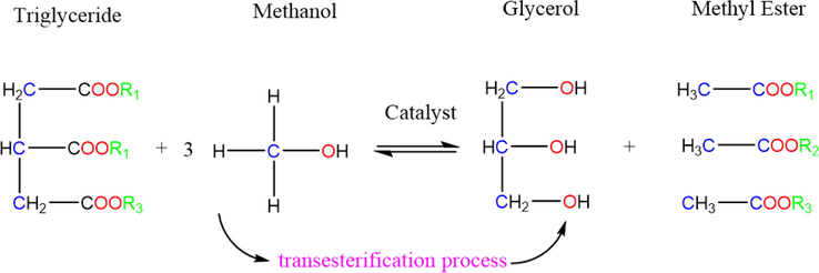
Representation of chemical reaction.
In production of different biodiesels various operating factors are important such as the temperature and pressure of process, the concentration, and type of catalyst, the molar ratio of alcohol to oil and the process time (Panchal, 2020; Pullen and Saeed, 2015; Rashid and Anwar, 2008). Therefore, optimizing these variables is very important to provide the maximum the biodiesel production yield (Nayak and Vyas, 2019; Panchal, 2020). However, many researchers use the conventional approach for optimization as varying one factor at a time while other parameters are constant, but this method is not appropriate because it is much cost and time consuming (Marwaha, 2019).
The rapid advancement of information technology has resulted in the generation of extremely huge number of datasets in fields such as science, medicine, sports and so on. These datasets may be too large or even too small for humans to process in a reasonable amount of time and find some real patterns and rules among them. As a result, various algorithms, meta-algorithms and other tools for identifying patterns and creating models are being created (Dean, 2014; Maimon and Rokach, 2009). These algorithms are part of a subset of AI known as Machine Learning (ML), which is defined as the study of methods and models that enable computer systems to complete a task (regression, classification, clustering or …) by learning from available data rather than being explicitly programmed (Makridakis et al., 2018; Ferrari-Trecate, 2003). ML tools excel at evaluating multidimensional data and allow for the creation of surrogate models that characterize enormous datasets. Self-driving cars, picture classification, audio recognition, natural language processing, and other high-dimensional data-driven breakthroughs have been enabled by ML technology (Yang, 2019).
The descriptor/feature is the input data to the ML model, and the label/ground truth is the desired property. There are three different approaches in machine learning: supervised, unsupervised, and reinforcement learning. Both data and labels are provided in supervised learning, and the model learns the mapping between the input features and the predicted output (classification and regression). Only the input is provided in unsupervised learning, and the model learns the shared characteristics and variations between the input data before grouping the data (clustering) (Grauman and Darrell, 2006).
Also, in reinforcement learning (Wiering and Van Otterlo, 2012), a model conducts actions depending on the current state, and the environment rewards (white cards) or punishes (red cards) the behavior. The agent will learn how to get more rewards and fulfill the assigned objective in its surroundings over time (Selvaratnam and Koodali, 2021).
The multilayer perceptron (MLP) is a well-known form of ANN that has several applications, including machine learning and pattern recognition. An input layer, multiple hidden layers, and an output layer are the various layers are in an MLP. After calculating a weighted sum of its inputs, each node in the network feeds this sum into a nonlinear activation function so that it can be used to generate an output. MLPs are capable of learning complex relationships between inputs and outputs, and can be trained using various algorithms such as backpropagation, which adjusts the weights of the network to minimize the error between the predicted and actual outputs (Venkatesan and Anitha, 2006).
Gradient boosting is another model that was chosen. Boosting technologies are a subset of ensemble algorithms that are distinct from bagging. The key concept of bagging ensemble algorithms (such as gradient boosting and adaptive boosting) is to expand the diversity of input samples of individual base (weak) learners through resampling capabilities, hence raising the predictability of the ensemble boosting approach. The basic principle of bootstrapping ensemble methods is to use the base learners to iteratively and step-by-step minimize the loss function until it achieves a specified limit (Natekin and Knoll, 2013).
The Gaussian process regression (GPR) is a popular ML model utilized in machine learning for modeling and predicting functions (Grbić et al., 2013). This approach is non-parametric and Bayesian, and it models the output function as a distribution of functions. In GPR, the data points are supposed to follow a multivariate Gaussian distribution, and the covariance between data points is modeled using a covariance function, also known as a kernel function. The kernel function specifies how the inputs are related to each other and can be chosen based on prior knowledge of the problem or learned from the data. The output of GPR is a distribution over functions, which can be used to make predictions with uncertainty estimates. GPR is commonly used in applications such as regression and classification, where the objective is to model and predict the behavior of complex systems or processes (Trapp, 2020; Wilson et al., 1110).
In this study, for the first time a comprehensive study of biodiesel production from Papaya oil was performed from computational point of view. Several ML models, including Multi-layer perceptron (MLP), Gradient Boosting with DT (GBDT), and Gaussian process regression (GPR), were employed to estimate the efficiency of producing biodiesel from Papaya oil methyl ester (POME). To achieve this, various important transesterification parameters were identified as input variables for the models, including reaction temperature (℃), sodium hydroxide concentration (NaOH, wt. %), treatment time (min), and methanol to papaya oil molar ratio.
2 Data for modeling and optimization of process
The experimental and coded values of selected operating factors for prediction of POME production yield are mentioned in Table 1. The data have been taken from a published source and more details about the experiments can be found in (Nayak and Vyas, 2019).
No.
(X1) Temperature,0C
(X2) Catalyst wt.%
(X3) Time, minute
(X4) Molar ratio
POME (Papaya oil methyl ester) yield (Y)
1
60
0.5
5.5
9
71
2
65
1.25
8
12
67
3
55
0.75
8
6
58
4
60
1
5.5
9
98.8
5
60
1
5.5
9
93
6
65
0.75
3
6
63
7
60
1
5.5
9
93.2
8
55
0.75
8
12
78.22
9
55
1.25
8
6
62
10
50
1
5.5
9
52
11
55
1.25
3
6
61
12
65
1.25
3
12
86
13
55
1.25
8
12
57
14
55
1.25
3
12
61
15
60
1
0.5
9
89.2
16
60
1.5
5.5
9
55
17
65
0.75
8
6
59
18
65
1.25
8
6
60
19
55
0.75
3
6
58
20
60
1
5.5
15
67
21
60
1
5.5
9
96
22
60
1
5.5
9
99
23
55
0.75
3
12
72.67
24
65
0.75
8
12
98.3
25
70
1
5.5
9
79
26
60
1
5.5
3
47
27
65
0.75
3
12
96
28
60
1
10.5
9
90
29
60
1
5.5
9
98.8
30
65
1.25
3
6
76.4
We have four independent variables in our regression problem: temperature, catalyst amount, time, and the molar ratio of methanol to oil. The only outcome of our regression problem is POME (Papaya oil methyl ester) yield (Y), and the only input variable is temperature °C. The whole dataset is depicted in Table 1. The experimental data used in this research are identical to those used in prior studies such as (Nayak and Vyas, 2019).
3 Methodology of optimization
3.1 Gaussian process regression model (GPR)
Gaussian process regression (GPR) is a machine learning technique that is widely used for modeling and predicting the behavior of complex systems. It is a Bayesian approach that can handle both linear and nonlinear regression problems, and has the added advantage of providing a measure of uncertainty in its predictions (Rasmussen, 2004).
At the heart of GPR lies the concept of the Gaussian process. In other words, a Gaussian process could be thought of as a probability distribution over functions, where each function is itself a random variable. The covariance function, k(x,x'), and the mean function, m(x), which describes the covariance between any pair of data points × and x', entirely defines the Gaussian process.
Given a set of N input–output pairs,
for
, the objective of GPR is to extract a function that maps inputs to outputs, while also providing a measure of uncertainty in its predictions. This is done by assuming that the outputs y are related to the inputs x through a Gaussian process, that is shown in Eq. (1).
In practice, it is common to choose a covariance function that accurately reflects the underlying structure of the data while setting the mean function to zero.
To train the Gaussian process, we need to estimate the parameters of the covariance function, which control the shape and behavior of the function. Finding the values of the parameters that maximize the log-likelihood of the data, as in Eq. (2), is the standard method for maximizing the likelihood of the data given the model parameters.
In the above equation, y stands for the vector of outputs, K is the N × N covariance matrix, and T denotes the determinant of a matrix.
Once the covariance function parameters have been estimated, we can use the Gaussian process to make predictions at new input locations. Specifically, given a new input x* and its associated covariance matrix K*, the predicted output is given by Eq. (3).
where I represents the identity matrix, stands for the noise variance, and y denotes the vector of actual outputs. The variance of the prediction at x* is given by Eq. (4).
Where, K** is the covariance between x* and itself.
3.2 MLP algorithm
The Multilayer Perceptron (MLP) model is widely utilized for ANN models in various kinds of applications. It has several levels of concealment, plus an input and an output layer. This architecture for the MLP method is often preferred due to its practicality and effectiveness in various applications (Rohani et al., 2011). The function that determines the activity of the neuron should be differentiable and non-decreasing in order to be considered a soft nonlinearity. Here, two different transfer functions were utilized, including the hyperbolic tangent (tanh) (Taki, 2016):
Beside the log-sigmoid (Taki, 2016):
The neural network is responsible for mapping vectors.
The goal is to adjust the network parameters so that the real output closely approximates the corresponding observed output ( ). The training procedure relies on minimizing some form of error cost (Taki, 2016). During the course of this investigation, we made use of Basic Backpropagation (BB) in conjunction with two separate training methods (Bayesian regularization backpropagation and Levenberg-Marquardt backpropagation). The first layer did not have any transfer functions, but the hidden layers were given sigmoid function applications. The output layer also made use of a linear transfer function so that it could make accurate predictions regarding the issues.
3.3 Gradient boosting (GB)
Gradient Boosting is boosting algorithm with the decision trees as core models. Gradient Boosting uses a statistical approach called boosting to improve standard decision tree models. The objective is to combine a set of base models to build a single strong model (Lin et al., 2012). The Gradient Boosting (GB) technique incrementally constructs new decision trees by reducing the current residuals. This iterative process optimizes the estimation by sequentially adding a new tree that minimizes the loss function. GB is essentially a functional gradient descent technique (Elith et al., 2008). Assume for the training set, for the loss function, and M for the count of iterations. GB in general works with these steps:
-
-
For m in {1,….M} Do:
In recent equations,
denotes the weight factor and
stands for the value of negative gradient calculated employing the prior model. The GBR workflow begins with an initial model f0(x), which implies M base models of decision trees to be created. For each iteration
, compensation of the residues is analogous to optimize the expansion coefficients
and
:
That gets:
AdaBoost (Schapire, 2013), LogitBoost (Li, 1203), and L2Boosting (Lutz et al., 2008) are just a few of the smooth loss functions supported by the gradient boosting framework (Bühlmann and Yu, 2003). Because of its simplicity and coherence, the squared loss function is used for this regression problem:
4 Results and discussion
To review and evaluate the performances of the proposed models with the data, the tuned hyper-parameters as described, and the final models are obtained using the explained methodology. Some criteria from the literature were utilized to assess a model's performance. Mean Absolute Percentage Error (MAPE), Root Mean Squared Error (RMSE), and R2 score are some of the criteria. The following are the statistical parameters (Taki, 2016):
where is the ith observed output for the jth pattern, stands for the predicted (from models) output for the jth pattern.
Also, and denote the mean of the entire observed and estimated values, respectively. Also, n stands for the size of dataset.
The size of the hidden layers may be the most crucial hyper-parameter for MLP. As shown in Fig. 1, the error rate is minimized in two intervals, and in order to keep the models simple, we selected a lesser quantity, which is comparable to 100.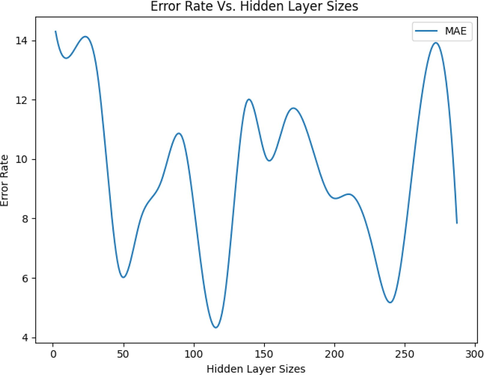
Change of Error Rate on Hidden Layer Sizes changes (MLP Model).
For other parameters, the optimized values are given in Table 2. To be more specific, the rectified linear unit (ReLU) function is utilized as the activation function for the hidden layer, which computes f(x) = max (0, x). Also, the weight optimization solver was chosen to be 'lbfgs,' which is a quasi-Newton technique optimizer.
Parameter
Value
Hidden layer sizes
104
activation
relu
solver
lbfgs
tol
0.027
There are not many parameters for tuning for the GPR model. The final configuration used in this model is presented in Table 3.
Parameter
Value
alpha
3.2e-07
Number of restarts optimizer
2
The optimized configuration for the GBDT model is also shown in Table 4.
Parameter
Value
Learning Rate
1.85
Number of estimators
60
loss
huber
criterion
mae
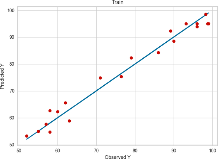
Examining Fig. 3, we can conclude that GPR performed very accurately in the learning phase since most of the observed and predicted values are very close to each other. When we put this fact together with Figs. 2 and 4, we can see that although the observed values differ from the predicted values in the test phase, they are in a reasonable neighborhood, which indicates a robust model.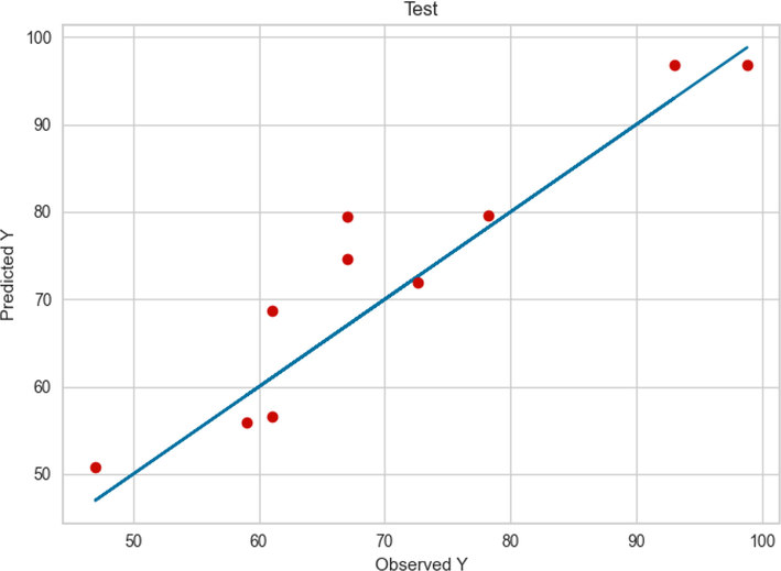
Comparison between the observed and model predicted values of POME using the GPR method on test data.
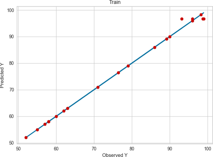
Comparison between the observed and model predicted values of POME using the GPR method on train data.
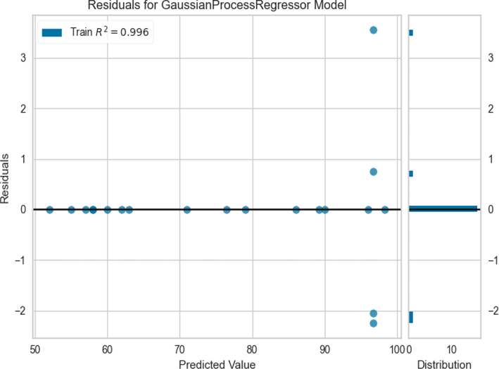
Residuals of prediction using GPR model.
Unlike the GPR model, many data points are not closely viewed during the MLP learning phase. The fact shown in Fig. 6 leads to poorer performance in the test phase, which is clearly visible in Fig. 5. Given these facts and the lack of convergence seen in Fig. 7 in MLP microwaves, this model is clearly inferior to GPR in terms of performance.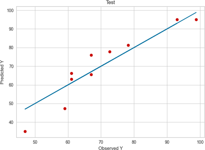
Comparison between the observed and model predicted values of POME using the MLP method on test data.
Comparison between the observed and model predicted values of POME using the MLP method on train data.
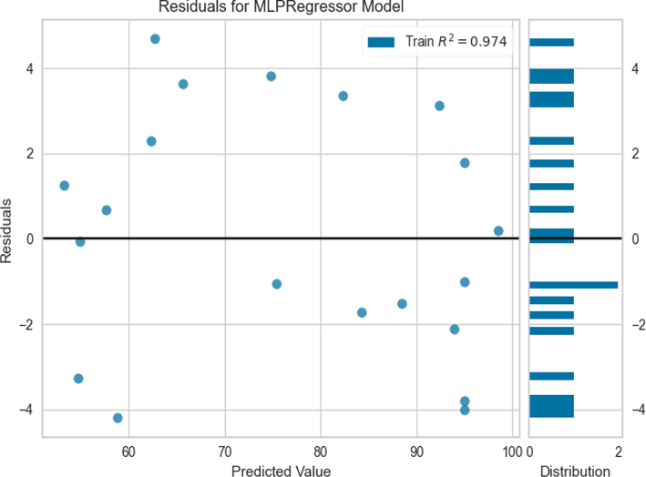
Residuals of prediction using MLP model.
The GBDT model has a performance close to the GPR model in terms of the learning phase, as can be seen in Fig. 9, so it has better accuracy than the MLP. This fact can be confirmed by Fig. 10 as well as the square R score shown in this figure. But as we can clearly see from Fig. 8, in some data points the predicted values are far from the observed values. This is a fact of this model being less general than the GPR model.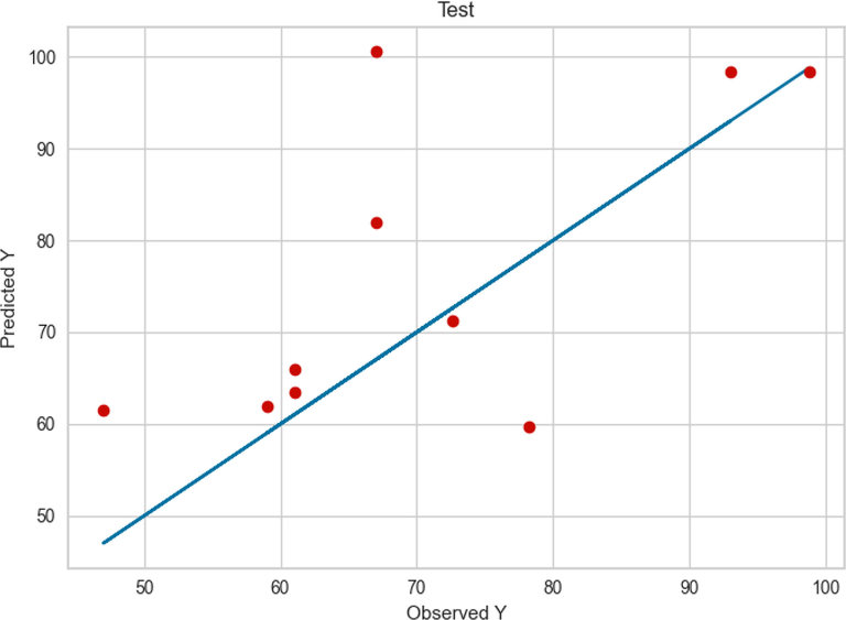
Comparison between the observed and model predicted values of POME using the GBDT method on test data.
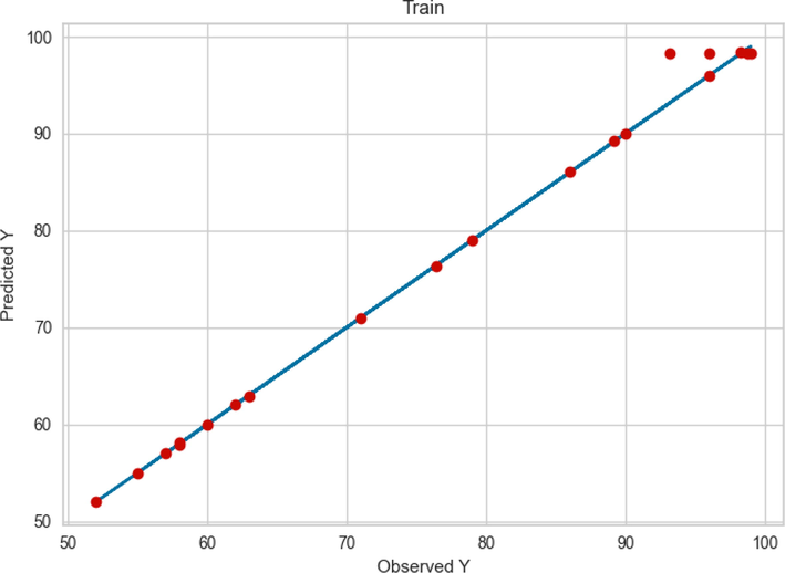
Comparison between the observed and model predicted values of POME using the GBDT method on train data.
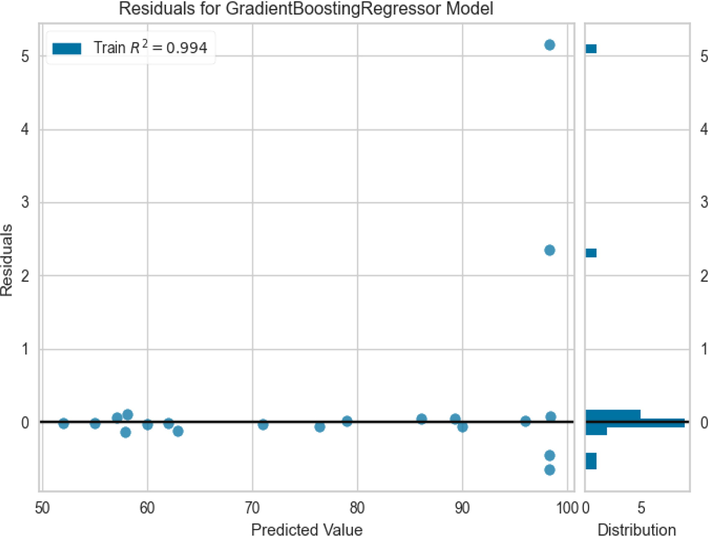
Residuals of prediction using GBDT model.
Based on the facts and figures that have been brought so far. The GPR model has a total equilibrium both in terms of generality and accuracy and looks better than the other two.
As a result of what has been mentioned in Table 5, the GPR model may be said to have the most practical experience with the proposed method in this research. As a result, to analyze the results of this model in greater depth, the effect of inputs on outputs is examined in two separate ways, as seen in the three-dimensional diagrams that follow.
Models
MAE
R2
MAPE
MLP
5.53360
0.97134
8.9670E-02
GPR
4.70105
0.9961
7.2080E-02
GBDT
1.32080E + 01
0.9893
2.0324E-01
The yield of product from Papaya oil is shown to vary as a result of the effect of various operational parameters in Figs. 11-16. As can be seen, Figs. 11-13 represent the predicted results of POME (Y) yield vs. the T against different parameters such as catalyst dose, treatment time, and methanol to Papaya oil molar ratio, respectively. As can be inferred by increasing the T factor (X1) to about 65 degree (Fig. 11), the yield of POME production increase while higher increasing the reaction temperature reduced the POME very fast (Jin, 2022). Therefore, it is very necessary to find the optimum value of this parameter. The same trend was observed in increasing the catalysts amount (X2). The POME production yield (Y) was in its optimum values when 0.875 wt% of catalyst was used in the reaction media. Fig. 12 shows the POME production yield vs. the reaction temperature and time reaction (X3). Increasing the reaction time from the beginning of the process until about 6.5 min, increased the yield of reaction. The exact optimum value for the process time was calculated to be 6.43 min. Finally, Fig. 13 displays the changes in the POME production yield by changing the amount of molar ratio of methanol to Papaya oil (X4) and the temperature of reaction. According to these results increasing the molar ratio led to an increment in POME and the optimum value for maximum production yield was calculated to be 10.875.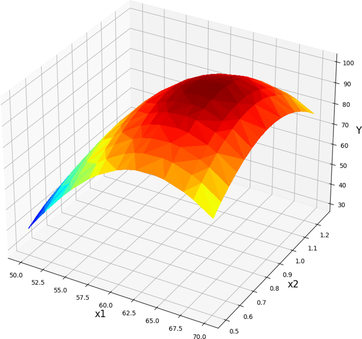
Projection of X1 and X2 with prediction surface in final GPR model. X3 = 5.5 and X4 = 12. Optimal value is 99.84 for X1 = 64 and X2 = 0.875.
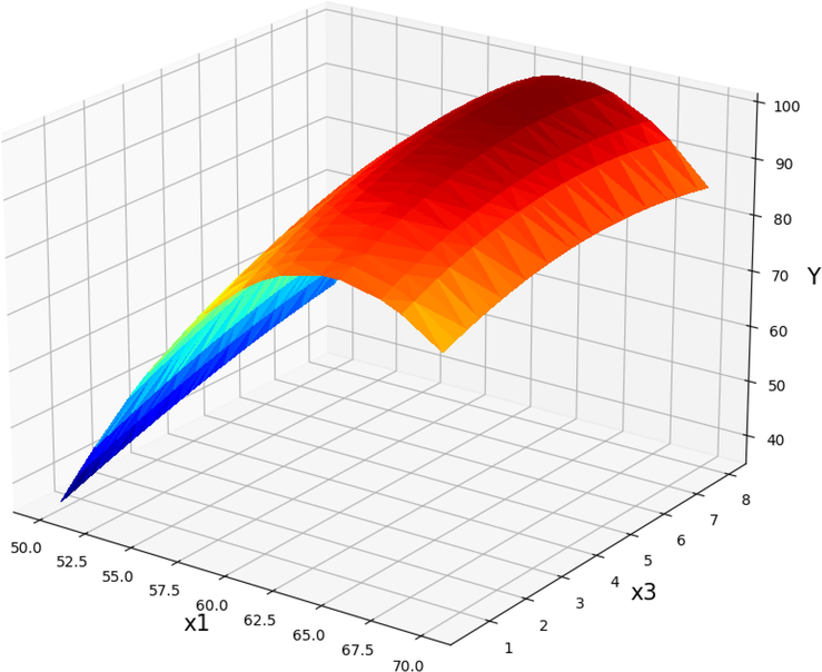
Projection of X1 and X3 with prediction surface in final GPR model. X2 = 0.75 and X4 = 12. Optimal value is 99.56 for X1 = 64 and X3 = 6.43.
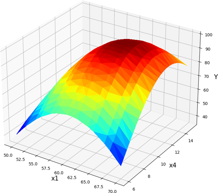
Projection of X1 and X4 with prediction surface in final GPR model. X2 = 0.75 and X3 = 5.5. Optimal value is 99.95 for X1 = 62 and X4 = 10.875.
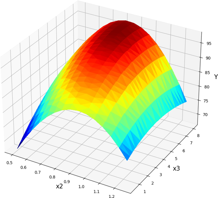
Projection of X2 and X3 with prediction surface in final GPR model. X1 = 60 and X4 = 12. Optimal value is 97.99 for X2 = 0.875 and X3 = 6.437.
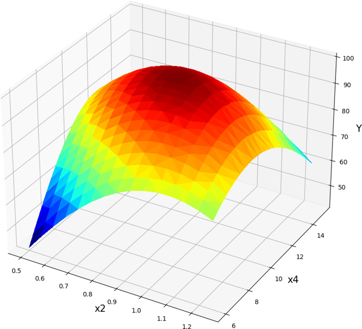
Projection of X2 and X4 with prediction surface in final GPR model. X1 = 60 and X3 = 5.5. Optimal value is 99.90 for X2 = 0.928 and X4 = 10.125.
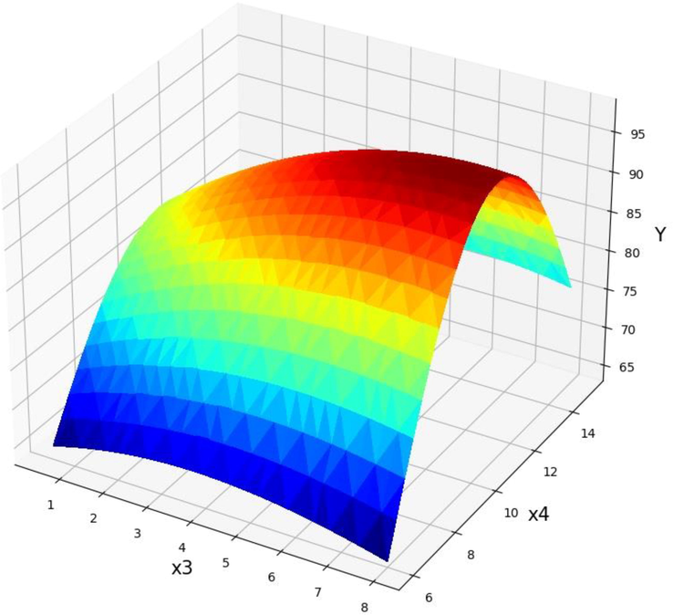
Projection of X3 and X4 with prediction surface in final GPR model. X1 = 60 and X2 = 0.75. Optimal value is 98.34 for X3 = 7.375 and X4 = 10.875.
The impact of the catalyst concentration (X2, NaOH) and the methanol to Papaya oil molar ratio (X4) on the POME efficiency is shown in Fig. 14. An increase in the catalyst content up to about 0.9 wt% resulted in the gradual increase in POME efficiency (Y) while other parameters were constant (X1 = 60 and X4 = 12). However, the higher increase of catalyst content the POME efficiency was decreased. As can be seen from Figs. 15 and 16 an increase in the molar ratio of methanol to papaya oil (X4) up to 10.87 resulted in the gradual increase in POME efficiency (Y) but after that POME efficiency production decreased. The dual effect of parameters on the POME production yield were observed in each 3D diagram while the two other parameters were kept at their constant values. By applying the investigated model to the range of available data, the optimal output values were obtained which are mentioned in Table 6.
Temperature,0C (X1)
Catalyst wt.% (X2)
Time, minute (X3)
Molar ratio
(X4)
Papaya oil methyl ester (POME) yield (Y)
64
0.875
7.375
10.875
99.96
5 Conclusion
Machine learning investigation of transesterification of Papaya oil for production of biodiesel was performed using three models including GPR, MLP, and GBDT. According to our findings, the GPR model has demonstrated superior accuracy and generalizability and can therefore be deemed the optimal choice. This method had 7.208E-02 and 4.701 errors according to MAPE and MAE criteria and also the R2 score in this model was estimated to be 0.996. The MAPE criterion, the MLP, GBDT models show error rates of 8.9670E-02, and 2.0324E-01, respectively. Due to the accuracy that has been maintained in generalization, this complete model can be considered as free from over-fitting, which can be considered as a complete model for this prediction, considering the available accuracy. According to the obtained results, increasing the operating values led to an improvement in the POME production yield. However, further increment of these values reduced the production yield. The optimum value of the highest POME yield production (Y) with the proposed method was estimated to be 99.96 %, with the details of 64 (⁰C) for temperature reaction (X1), 0.875 wt% catalyst amount (X2), reaction time (X3) of 6.433 min, and 10.875 of methanol to Papaya oil molar ratio (X4).
Acknowledgement
This study is supported via funding from Prince Sattam bin Abdulaziz University project number (PSAU/2023/R/1444).
Declaration of Competing Interest
The authors declare that they have no known competing financial interests or personal relationships that could have appeared to influence the work reported in this paper.
References
- The effects of catalysts in biodiesel production: A review. J. Ind. Eng. Chem.. 2013;19(1):14-26.
- [Google Scholar]
- Boosting with the L 2 loss: regression and classification. J. Am. Stat. Assoc.. 2003;98(462):324-339.
- [Google Scholar]
- Experimental and numerical investigation of the effect of fig seed oil methyl ester biodiesel blends on combustion characteristics and performance in a diesel engine. Energy Rep.. 2021;7:5846-5856.
- [Google Scholar]
- Big data, data mining, and machine learning: value creation for business leaders and practitioners. John Wiley & Sons; 2014.
- A clustering technique for the identification of piecewise affine systems. Automatica. 2003;39(2):205-217.
- [Google Scholar]
- Grauman, K. and T. Darrell. Unsupervised learning of categories from sets of partially matching image features. in 2006 IEEE Computer Society Conference on Computer Vision and Pattern Recognition (CVPR'06). 2006. IEEE.
- Stream water temperature prediction based on Gaussian process regression. Expert Syst. Appl.. 2013;40(18):7407-7414.
- [Google Scholar]
- Optimization and analysis of bioenergy production using machine learning modeling: Multi-layer perceptron, Gaussian processes regression, K-nearest neighbors, and Artificial neural network models. Energy Rep.. 2022;8:13979-13996.
- [Google Scholar]
- The optimal share of wave power in a highly renewable power system on the Iberian Peninsula. Energy Rep.. 2016;2:221-228.
- [Google Scholar]
- Li, P., Robust logitboost and adaptive base class (abc) logitboost. arXiv preprint arXiv:1203.3491, 2012.
- Estimation of battery state of health using probabilistic neural network. IEEE Trans. Ind. Inf.. 2012;9(2):679-685.
- [Google Scholar]
- Introduction to knowledge discovery and data mining. In: Data mining and knowledge discovery handbook. Springer; 2009. p. :1-15.
- [Google Scholar]
- Statistical and Machine Learning forecasting methods: Concerns and ways forward. PLoS One. 2018;13(3):e0194889.
- [Google Scholar]
- Biodiesel production from Terminalia bellerica using eggshell-based green catalyst: An optimization study with response surface methodology. Energy Rep.. 2019;5:1580-1588.
- [Google Scholar]
- Optimization of microwave-assisted biodiesel production from Papaya oil using response surface methodology. Renew. Energy. 2019;138:18-28.
- [Google Scholar]
- Optimization of soybean oil transesterification using an ionic liquid and methanol for biodiesel synthesis. Energy Rep.. 2020;6:20-27.
- [Google Scholar]
- Investigation of the factors affecting the progress of base-catalyzed transesterification of rapeseed oil to biodiesel FAME. Fuel Process. Technol.. 2015;130:127-135.
- [Google Scholar]
- Production of biodiesel through optimized alkaline-catalyzed transesterification of rapeseed oil. Fuel. 2008;87(3):265-273.
- [Google Scholar]
- Gaussian processes in machine learning. Springer; 2004.
- Prediction of tractor repair and maintenance costs using Artificial Neural Network. Expert Syst. Appl.. 2011;38(7):8999-9007.
- [Google Scholar]
- Machine learning in experimental materials chemistry. Catal. Today. 2021;371:77-84.
- [Google Scholar]
- Heat transfer and MLP neural network models to predict inside environment variables and energy lost in a semi-solar greenhouse. Energ. Buildings. 2016;110:314-329.
- [Google Scholar]
- Modeling and experimental validation of heat transfer and energy consumption in an innovative greenhouse structure. Information Processing in Agriculture. 2016;3(3):157-174.
- [Google Scholar]
- Deep structured mixtures of gaussian processes. In: International Conference on Artificial Intelligence and Statistics. PMLR; 2020.
- [Google Scholar]
- Application of a radial basis function neural network for diagnosis of diabetes mellitus. Curr. Sci.. 2006;91(9):1195-1199.
- [Google Scholar]
- Wilson, A.G., D.A. Knowles, and Z. Ghahramani, Gaussian process regression networks. arXiv preprint arXiv:1110.4411, 2011.
- Concepts of artificial intelligence for computer-assisted drug discovery. Chem. Rev.. 2019;119(18):10520-10594.
- [Google Scholar]
- A comparative study on the effect of unsaturation degree of camelina and canola oils on the optimization of bio-diesel production. Energy Rep.. 2016;2:211-217.
- [Google Scholar]


