

Translate this page into:
Novel numerical simulation of drug solubility in supercritical CO2 using machine learning technique: Lenalidomide case study
⁎Corresponding author. r.zhrani@tu.edu.sa (Rami M. Alzhrani)
-
Received: ,
Accepted: ,
This article was originally published by Elsevier and was migrated to Scientific Scholar after the change of Publisher.
Peer review under responsibility of King Saud University.
Abstract
In pharmaceutical industry, finding promising ways to enhance the solubility of disparate types of drugs is an important challenge for the orally administered drug delivery system. Disparate techniques based on drug characteristics, nature of dosage form and properties of excipients have recently been under extensive evaluation all over the world to improve the solubility of poorly water-soluble drugs. Among them, supercritical fluid carbon dioxide (SC-CO2) has received paramount attentions due to having considerable advantages like cost-effectiveness and low flammability. Lenalidomide belongs is an orally administered anti-cancer agent, which has recently received indication for the treatment of adult patients with different bone marrow-related malignancies such as multiple myeloma, mantle cell lymphoma and follicular lymphoma. Predicting the optimized value of Lenalidomide inside the SC-CO2 in a wide range of pressure and temperature via developing mathematical models based on artificial intelligence (AI) is the main objective of this paper. In this study, three different machine learning based models are selected to predict and optimized the drug solubility. The available data includes 28 rows of data with two inputs including temperature and pressure and two outputs including density and solubility. Selected models are Kernel Ridge Regression (KRR), least angle regression (LAR), and Multilayer Perceptron (MLP). After optimizing models and comparing the results, the MLP was selected as the primary model of this research. The models illustrated R-squared scores of 0.999 and 0.994 for density and solubility. The maximum errors are also 2.92 and 6.44 × 10⁻² for these outputs, which shows the accuracy and significant generality of the model.
Keywords
Supercritical fluid
Solubility Optimization
Lenalidomide
Numerical modeling

1 Introduction
A determinative parameter in pharmaceutical industry, which significantly affects the performance and efficiency of a developed medicine is drug solubility (Kneller, 2010; Drews and Ryser, 1997; Padervand, 2017). This parameter possesses an incontrovertible role in specifying the desired concentration of a drug to obtain the necessary pharmacological response (Nguyen, 2022; Batchelor, 2022; Padervand et al., 2020).
With the aim of increasing drug solubility, various techniques including particle size reduction, application of surfactants, supercritical fluids (SCFs) and solid dispersion have been employed (Sareen et al., 2012; Girotra et al., 2013; Chaudhari and Dugar, 2017; Padervand et al., 2021). Among the approaches, the application of carbon dioxide SCF (SC-CO2) has been more attractive after 1980 s due to its encouraging properties such as low cost, simplicity of use and low toxicity/flammability (Hannay and Hogarth, 1880; Dohrn, 2007; Padervand and Elahifard, 2017).
Lenalidomide (Revlimid®) is a well-known antineoplastic/angiogenesis inhibitor, which has received various indications by the U.S food and drug administration (FDA) and the European medicines agency (EMA) for the treatment of adult patients suffering from certain types of bone marrow-related malignancies such as multiple myeloma and myelodysplastic syndromes (MDS) (Padervand, 2021). Table 1 comprehensively renders the molecular structure and properties of Lenalidomide (Palumbo, 2012; Zeldis, 2011).
Molecular structure
Chemical formula
CAS number
Molecular weight
Route of administration
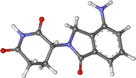
C13H13N3O3
191732–72-6
259.265 g·mol−1
Oral
Machine learning (ML) is an artificial intelligence (AI) discipline that consists of a set of techniques that aid in the comprehension of patterns in data without making any assumptions about the data's structure. Building nonlinear correlations in data, as well as the interaction between predictors, is one of these methodologies' strengths (Senders, 2018; Cherkassky and Ma, 2003; Carbonell et al., 1983; Goodfellow et al., 2016). In this research, three approaches are selected as a novel approach to make models on the solubility dataset using Python (3.9) software. Selected models are Kernel Ridge Regression (KRR), Least angle regression (LAR), and Multilayer perceptron (MLP). Those models have been used as a novel method for the first time to optimize the solubility of Lenalidomide.
Least Angle Regression provides linear regression model coefficient routes with understandable geometrical interpretation. LAR's solution routes are piecewise linear and hence highly efficient to compute. This gives the algorithm with tremendous computational benefits over other variable selection approaches. LAR selects the predictor variable which is most associated with the response variable, and a regression coefficient update proceeds in this manner, starting with all coefficients equal to 0 (Lee and Jun 2018; Madigan and Ridgeway, 2004).
The Kernel Ridge Regression employs both ridge regressions and the kernel technique (KRR). Through regularization and kernel approaches, KRR provides the benefit of capturing nonlinear connections while avoiding regression over-fitting concerns (McDonald, 2009; Zhang et al., 2013). Also, a nonlinear mapping between input and output vectors is examined by the multilayer perceptron. It is made up of basic linked components known as neurons or nodes. Each neuron has a straightforward task to complete (Mielniczuk and Tyrcha, 1993; Noriega, 2005).
3.Materials and Method.
In this section, we will discuss the data used as well as the models that have been used in this research as the main structure of the analysis performed in more detail.
1.1 Data set
The data set analyzed in this study, which is taken from (Sajadian, 2022), has 28 rows of data whose inputs are temperature and pressure and whose outputs are solubility and density, as shown in Table 2. For more visibility, the pairwise relationship of the parameters is visualized in Fig. 1. Also, the Pearson Correlation (PC) Plot and Kendall Correlation Plot are shown in Fig. 2.
No.
T (K)
P (bar)
Density (kg m−3)
Solubility (×104) (mole fraction)
1
308
120
768.42
0.17
2
308
150
816.06
0.22
3
308
180
848.87
0.31
4
308
210
874.40
0.36
5
308
240
895.54
0.45
6
308
270
913.69
0.56
7
308
300
929.68
0.70
8
318
120
659.73
0.09
9
318
150
743.17
0.17
10
318
180
790.18
0.30
11
318
210
823.71
0.39
12
318
240
850.10
0.51
13
318
270
872.04
0.67
14
318
300
890.92
0.83
15
328
120
506.85
0.04
16
328
150
654.94
0.14
17
328
180
724.13
0.31
18
328
210
768.74
0.44
19
328
240
801.92
0.58
20
328
270
828.51
0.80
21
328
300
850.83
0.94
22
338
120
384.17
0.02
23
338
150
555.23
0.10
24
338
180
651.18
0.32
25
338
210
709.69
0.52
26
338
240
751.17
0.72
27
338
270
783.29
0.93
28
338
300
809.58
1.08
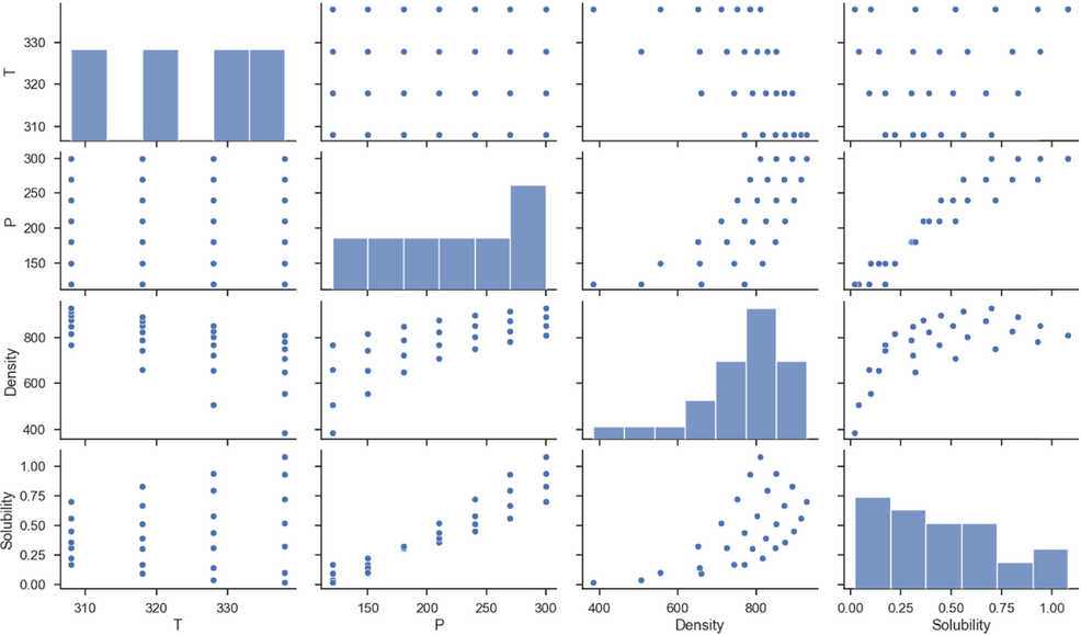
Pairwise Distribution.
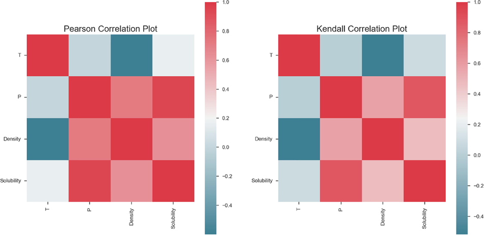
Correlation Plots.
1.2 Models
Least angle regression (LAR) (Efron, 2004) is an effective variable selection approach. Expressly, it aims to pick the predictors (in our example, the basis polynomials) which have the largest influence on the estimator response from a potentially vast range of alternatives. LAR ultimately produces a sparse PC approximation, i.e., one with fewer terms than a traditional complete representation.
More specifically, LAR gives a collection of PC representations, where the first meta-model comprises a single estimator, the second contains two estimators, and so on. Following that, a criterion for picking the “best” meta-model is presented. A cross validation routine is used to estimate the correctness of each meta-model generated by LAR. Eventually, the meta-model with the highest estimate is preserved. Its sparsity is substantially smaller than the cardinality of the entire candidate basis. Finally, adaptive procedures that rely on repetitions of the LAR procedure are described in full (Blatman and Sudret, 2011). The below algorithm summarizes the LAR regression steps:
-
Set the coefficients to .
-
Initialize residual to the Y vector of training data.
-
Find the vector that has the highest correlation with the present residual.
-
Change from 0 to the least square coefficient of the current residual on until another predictor has the same correlation with the current residual as .
-
Change a together in the direction given by their joint least square coefficient of the current residual on until some other predictor shows the same correlation with the current residual.
Go on this manner until m ≡ min (P, N − 1) estimators are entered.
The active coefficients are “moved” toward their least square value in steps 3 and 4. It is equivalent to amending the form (Efron, 2004; Khan et al., 2007).
The LAR descent direction and step are denoted by vector and coefficient γ(k). As shown, both values may be obtained algebraically. It is important to mention that if N ⩾ P, then the ordinary least-square solution is provided by the final stage of LAR.
Kernel ridge regression (KRR), the other approach employed, is centered on ridge regression and ordinary least squares (OLS) regression. Suppose a data set
is given and contains
data points pulled from an undetermined distribution
over
× ℝ. The objective is to predict a function that optimizes the MSE of the data [
], where the expectation is taken jointly over
pairs. The conditional mean
is widely accepted as the best function (Byrne and Schniter, 2016). To predict the undetermined function
, An alternative solution is to use an M−estimator with least squares loss over the dataset and a weighted penalty based on the squared Hilbert norm (Vovk, 2013);
In the above equation, greater than 0 is a regularization parameter and H indicates a reproducing kernel Hilbert space, the estimator is determined as the kernel ridge regression estimate, or KRR for short (Zhang et al., 2013). It is a natural non-parametric extension of the traditional ridge regression estimate (Hoerl and Kennard, 1970).
The multilayer perceptron analyzes a nonlinear mapping between input and output vectors. It comprises a group of simple interconnected units called neurons or nodes. There is a simple job that each neuron must do.
In contrast, neurons with many connections can solve complex and challenging problems that are not linear. Neurons are usually placed in layers. Multilayer Perceptron (MLP) is frequently used as an input layer, followed by numerous hidden layers, and finally an output layer. All these structures are called Multilayer Perceptron networks (Mucherino et al., 2009).
When paired with other training methods, the Levenberg–Marquardt algorithm produced the greatest accuracy when compared to gradient-based methods, and it was selected for network testing due to its quicker convergence. Sigmoid-log and tangent-sigmoid are the most often used model ANN activation functions, as is BP (Back Propagation). The input elements , weight , bias , and are represented in the following equations. Function or output is the value (Deo and Şahin, 2015).
These three models have some important hyper-parameters that we optimize them using Grid Search method that tests different combinations to find the best combination. These hyper-parameters are listed in Table 3. Alpha Fit intercept Alpha Fit intercept Solver Tolerance Hidden layer sizes Activation Solver Tolerance
Model
Hyper-Parameters
LAR
KRR
MLP
2 Results
To optimize models with their Hyper-parameters, different combinations examined, and the final models implemented. The final values are listed in Table 4. Alpha: 0.0009 Fit intercept: False Alpha: 0.1478 Fit intercept: True Alpha: 0.19653 Fit intercept: True Solver: sag Tolerance: 14.2303 Alpha: 0.01993 Fit intercept: True Solver: auto Tolerance: 12.7768 Hidden layer sizes: 32 Activation: relu Solver: lbfgs Tolerance: 0.00237 Hidden layer sizes: 28 Activation: logistic Solver: lbfgs Tolerance: 0.0245
Model
Hyper-Parameters for Solubility
Hyper-Parameters for Density
LAR
KRR
MLP
After tuning of models, the evaluation is done with multiple numeric and visual method. In Table 5 the R-square (Coefficient of Determination) scores of final models are displayed. This metric is used on a regression line to determine how close the predicted values are to the true (expected) values (Botchkarev, 2018).
Models / Output
Density
Solubility
KRR
0.416
0.957
LAR
0.682
0.875
MLP
0.999
0.994
Where, μ indicates the mean of the expected data. For solubility prediction both KRR and MLP methods have scores more than 0.95 but for density prediction the only accurate model is MLP.
Error Rates of models are also displayed in Table 6 with metrics such as Mean Absolute Error (MAE), Mean Absolute Percentage Error (MAPE), and Maximum Error (De Myttenaere, 2016; Paula, 2020):
Metric
Mean Absolute Error (MAE)
Root Mean Square Error (RMSE)
Mean Absolute Percentage Error (MAPE)
Max Error
output
Density
Solubility
Density
Solubility
Density
Solubility
Density
Solubility
KRR
4.37E + 01
5.92E-02
8.05E + 01
7.04E-02
9.54E-02
8.33E-01
1.97E + 02
1.16E-01
LAR
4.40E + 01
8.53E-02
7.58E + 01
1.00E-01
9.49E-02
9.41E-01
1.80E + 02
1.89E-01
MLP
1.30E + 00
1.80E-02
1.59E + 00
2.77E-02
2.23E-03
5.54E-01
2.92E + 00
6.44E-02
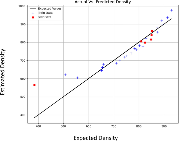
Figs. 3 to 8 schematically compare the expected and predicted values. In these figures, the black line shows the expected values, red squares indicate the test data and sign plus denotes the train data. According to Table 6, the MLP model has the least errors in all cases for both outputs. Also, in Figs. 3–8, the visual comparison of expected and predicted values is displayed. All these figures together confirm the fact that MLP is the most accurate and general model. Therefore, MLP was selected as the main model for both outputs in this study.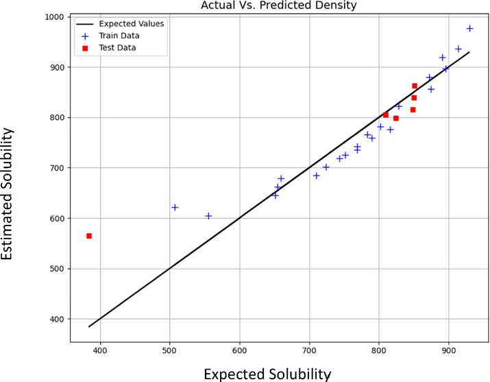
Expected vs Estimated values of Density (kg m−3) (KRR model).
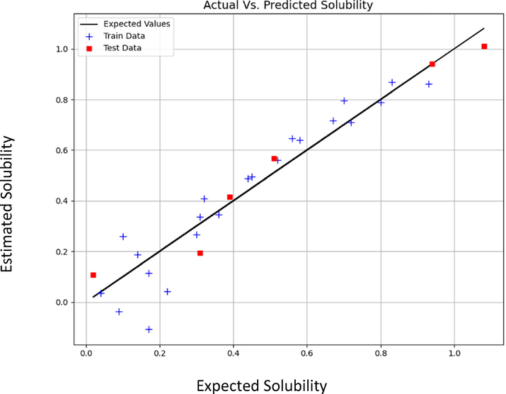
Expected vs Estimated values of Solubility (mole fraction) (KRR model).
Expected vs Estimated values of Density (kg m−3) (LAR model).
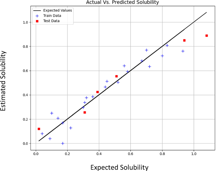
Expected vs Estimated values of Solubility (mole fraction) (LAR model).
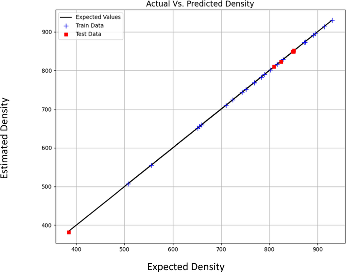
Expected vs Estimated values of Density (kg m−3) (MLP model).

Expected vs Estimated values of Solubility (mole fraction) (MLP model).
Figs. 9 and 10 demonstrate the simultaneous effects of temperature and pressure on the density and solubility of Lenalidomide based on MLP model. By looking at the figures, it can be understood that increment of pressure directly improves the Lenalidomide solubility in SC-CO2 system. Increment of pressure possesses encouraging impact on the density of solvent, which frequently improves the solvating strength of the SC-CO2 and thus, improves the solubility of drug. Despite the positive effect of pressure on the solubility of drugs, there is a paradoxical trend in the connection of temperature and solubility. As can be seen in Figs. 11, 12, 13 and 14, increase in pressure results in a significant enhancement in the compactness of solvent, which is attributed to greater density and superior solvating power of SC-CO2 as solvent. With the aim of assessing the effect of temperature on Lenalidomide solubility, study on the role of two factors including sublimation pressure and density above and below the cross-over pressure (COP) is of prime importance. By increasing the temperature at the pressures above the COP, the positive effect of sublimation pressure on Lenalidomide solubility overcomes the destructive influence of density reduction by increasing temperature. In doing so, at the pressures above the COP, increase in the temperature significantly improves the solubility of drugs in SC-CO2 system. At the pressures less than the COP, the deteriorative effect of density decrement is greater than the encouraging impact of sublimation pressure. Thus, at these pressures, increment of the temperature dramatically declines the solubility Lenalidomide in SC-CO2 solvent (Alshehri, 2022).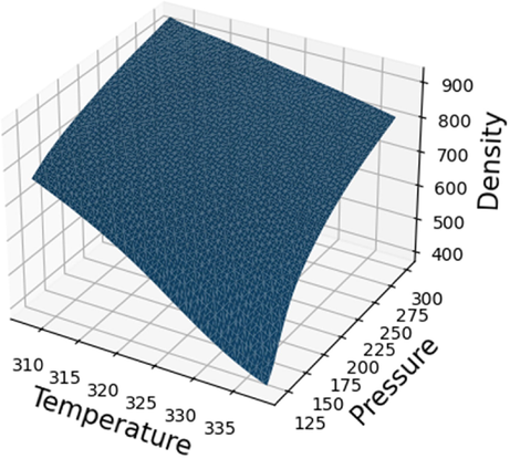
Final prediction surface for density.
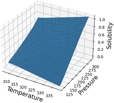
Final prediction surface for solubility.
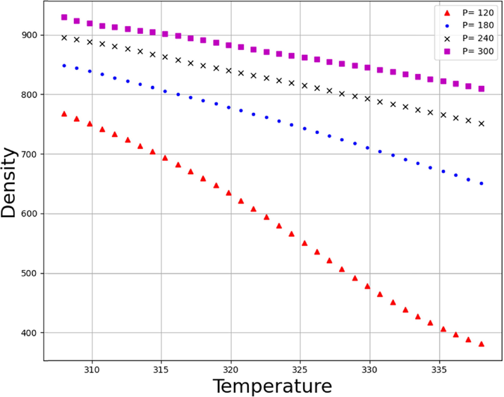
Density Trends of Temperature (K) on different values of Pressure (bar).
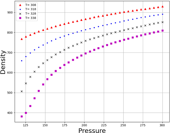
Density Trends of Pressure (bar) on different values of Temperature (K).
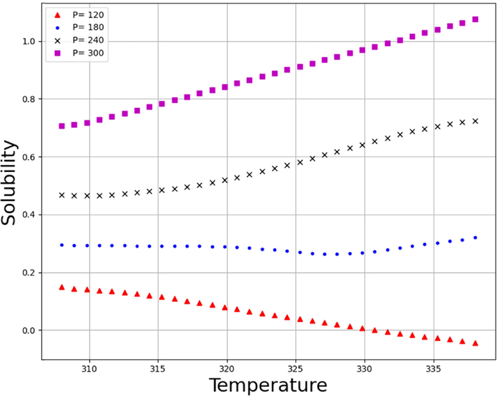
Solubility Trends of Temperature (K) on different values of Pressure (bar).
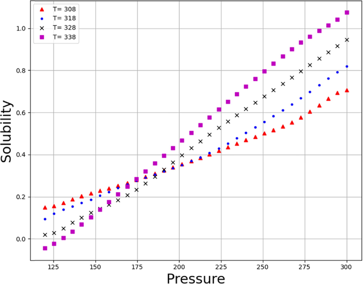
Solubility Trends of Pressure (bar) on different values of Temperature (K).
3 Conclusion
Application of SC-CO2 as a robust, cost-effective, and versatile solvent has been of great attention in current decades. The prominent objective of this research was applying machine learning (ML) models to investigate and create a model for the density and solubility of Lenalidomide in SC-CO2. The data that is currently available consists of 28 rows, including two inputs temperature and pressure. Both density and solubility are produced as the results. Kernel Ridge Regression (KRR), Least Angle Regression (LAR), and Multilayer Perceptron are some of the models that have been selected (MLP). The MLP was ultimately chosen as the primary model for this research after it was optimized and compared to several other models. The R-squared scores for our model are 0.999 for density and 0.994 for solubility. Both metrics are highly accurate. In addition, the maximum errors for these outputs are both 2.92 and 6.44 × 10⁻², which demonstrates both the precision and significant generality of the model. In terms of MAPE the model has error rate of 2.23 × 10⁻³on density and 5.54 × 10⁻¹ on solubility.
Acknowledgement
Rami M. Alzhrani would like to acknowledge Taif University Research Supporting Project Number (TURSP-2020/209), Taif University, Taif, Saudi Arabia.
Declaration of Competing Interest
The authors declare that they have no known competing financial interests or personal relationships that could have appeared to influence the work reported in this paper.
References
- Batchelor, H., 2022. Solubility. Biopharmaceutics: From Fundamentals to Industrial Practice, p. 39-50.
- Design of predictive model to optimize the solubility of Oxaprozin as nonsteroidal anti-inflammatory drug. Scientific Reports. 2022;12:13106 In this issue
- [CrossRef] [Google Scholar]
- Adaptive sparse polynomial chaos expansion based on least angle regression. J. Comput. Phys.. 2011;230(6):2345-2367.
- [Google Scholar]
- Botchkarev, A., 2018. Evaluating performance of regression machine learning models using multiple error metrics in azure machine learning studio. Available at SSRN 3177507.
- Sparse multinomial logistic regression via approximate message passing. IEEE Trans. Signal Process.. 2016;64(21):5485-5498.
- [Google Scholar]
- Application of surfactants in solid dispersion technology for improving solubility of poorly water soluble drugs. J. Drug Delivery Sci. Technol.. 2017;41:68-77.
- [Google Scholar]
- Comparison of model selection for regression. Neural Comput.. 2003;15(7):1691-1714.
- [Google Scholar]
- Mean absolute percentage error for regression models. Neurocomputing. 2016;192:38-48.
- [Google Scholar]
- Application of the extreme learning machine algorithm for the prediction of monthly Effective Drought Index in eastern Australia. Atmos. Res.. 2015;153:512-525.
- [Google Scholar]
- Melting point depression by using supercritical CO2 for a novel melt dispersion micronization process. J. Mol. Liq.. 2007;131:53-59.
- [Google Scholar]
- Drug Development: The role of innovation in drug development. Nat. Biotechnol.. 1997;15(13):1318-1319.
- [Google Scholar]
- File:Lenalidomide ball-and-stick.png. (2020, September 16). Wikimedia Commons, the free media repository. Retrieved 12:42, June 6, 2022 from https://commons.wikimedia.org/w/index.php?title=File:Lenalidomide_ball-and-stick.png&oldid=461504637.
- Supercritical fluid technology: a promising approach in pharmaceutical research. Pharm. Dev. Technol.. 2013;18(1):22-38.
- [Google Scholar]
- I. On the solubility of solids in gases. Proc. R. Soc. London. 1880;30(200–205):178-188.
- [Google Scholar]
- Ridge regression: Biased estimation for nonorthogonal problems. Technometrics. 1970;12(1):55-67.
- [Google Scholar]
- Robust linear model selection based on least angle regression. J. Am. Stat. Assoc.. 2007;102(480):1289-1299.
- [Google Scholar]
- The importance of new companies for drug discovery: origins of a decade of new drugs. Nat. Rev. Drug Discovery. 2010;9(11):867-882.
- [Google Scholar]
- Fast incremental learning of logistic model tree using least angle regression. Expert Syst. Appl.. 2018;97:137-145.
- [Google Scholar]
- Madigan, D., Ridgeway, G., 2004. Discussion of“ Least angle regression” by Efron et al. arXiv preprint math/0406469.
- Consistency of multilayer perceptron regression estimators. Neural Networks. 1993;6(7):1019-1022.
- [Google Scholar]
- K-nearest neighbor classification. In: Data Mining in Agriculture. Springer; 2009. p. :83-106.
- [Google Scholar]
- Computational prediction of drug solubility in supercritical carbon dioxide: Thermodynamic and artificial intelligence modeling. J. Mol. Liq.. 2022;354:118888
- [Google Scholar]
- Multilayer perceptron tutorial. School of Computing: Staffordshire University; 2005.
- Reverse phase HPLC determination of sunitinib malate using UV detector, its isomerisation study, method development and validation. J. Anal. Chem.. 2017;72(5):567-574.
- [Google Scholar]
- Preferential Solvation of Pomalidomide, an Immunomodulatory Drug, in Some Biocompatible Binary Mixed Solvents at 298.15 K. Russ. J. Phys. Chem. A. 2021;95(12):2432-2443.
- [Google Scholar]
- Development of a spectrophotometric method for the measurement of kinetic solubility: economical approach to be used in pharmaceutical companies. Pharm. Chem. J.. 2017;51(6):511-515.
- [Google Scholar]
- Preferential solvation of pomalidomide, an anticancer compound, in some binary mixed solvents at 298.15 K. Chin. J. Chem. Eng.. 2020;28(10):2626-2633.
- [Google Scholar]
- Preferential solvation and solvation shell composition of sunitinib malate, an anti-tumor compound, in some binary mixed solvents at 298.15 K. Chem. Pap.. 2021;75(3):939-950.
- [Google Scholar]
- Continuous lenalidomide treatment for newly diagnosed multiple myeloma. N. Engl. J. Med.. 2012;366(19):1759-1769.
- [Google Scholar]
- Predicting Long-Term Wind Speed in Wind Farms of Northeast Brazil: A Comparative Analysis Through Machine Learning Models. IEEE Lat. Am. Trans.. 2020;18(11):2011-2018.
- [Google Scholar]
- Experimental analysis and thermodynamic modelling of lenalidomide solubility in supercritical carbon dioxide. Arabian J. Chem.. 2022;15(6):103821
- [Google Scholar]
- Improvement in solubility of poor water-soluble drugs by solid dispersion. Int. J. Pharm. Invest.. 2012;2(1):12.
- [Google Scholar]
- Trial watch: lenalidomide-based immunochemotherapy. Oncoimmunology. 2013;2(11):e26494.
- [Google Scholar]
- Machine learning and neurosurgical outcome prediction: a systematic review. World Neurosurg.. 2018;109:476-486.
- [Google Scholar]
- Wikipedia contributors. 2022, May 27. Lenalidomide. In Wikipedia, The Free Encyclopedia. Retrieved 12:48, June 6, 2022, from https://en.wikipedia.org/w/index.php?title=Lenalidomide&oldid=1090079965.
- A review of the history, properties, and use of the immunomodulatory compound lenalidomide. Ann. N. Y. Acad. Sci.. 2011;1222(1):76-82.
- [Google Scholar]
- Zhang, Y., Duchi, J., Wainwright, M., 2013. Divide and conquer kernel ridge regression. In: Conference on learning theory. PMLR.


