

Translate this page into:
Optimal control approach for nonlinear chemical processes with uncertainty and application to a continuous stirred-tank reactor problem
⁎Corresponding authors at: School of Mathematical Sciences, Guizhou Normal University, Guiyang 550001, PR China (X. Wu); School of Life Sciences, Guizhou Normal University, Guiyang 550001, PR China (Y.Z. Hou). xwu@gznu.edu.cn (Xiang Wu), yuzhou_hou@163.com (Yuzhou Hou)
-
Received: ,
Accepted: ,
This article was originally published by Elsevier and was migrated to Scientific Scholar after the change of Publisher.
Peer review under responsibility of King Saud University.
Abstract
Practical chemical process is usually a dynamic process including uncertainty. Stochastic constraints can be used to chemical process modeling, where constraints cannot be strictly satisfied or need not be fully satisfied. Thus, optimal control of nonlinear systems with stochastic constraints can be available to address practical nonlinear chemical process problems. This problem is hard to cope with due to the stochastic constraints. By introducing a novel smooth and differentiable approximation function, an approximation-based approach is proposed to address this issue, where the stochastic constraints are replaced by some deterministic ones. Following that, the stochastic constrained optimal control problem is converted into a deterministic parametric optimization problem. Convergence results show that the approximation function and the corresponding feasible set converge uniformly to that of the original problem. Then, the optimal solution of the deterministic parametric optimization problem is guaranteed to converge uniformly to the optimal solution of the original problem. Following that, a computation approach is proposed for solving the original problem. Numerical results, obtained from a nonlinear continuous stirred-tank reactor problem including stochastic constraints, show that the proposed approach is less conservative compared with the existing typical methods and can obtain a stable and robust performance when considering the small perturbations in initial system state.
Keywords
Optimal control
Nonlinear chemical processes
Stochastic constraints
Approximation function
Convergence analysis
Stirred-tank reactor

1 Introduction
It is well-recognized that the chemical process problem is a challenging control problem due to its nonlinear nature and the existence of system state and control input constraints (Braatz and Crisalle, 2007; Ostrovsky et al., 2012; Skogestad, 2004; Wang et al., 2011; Zheng et al., 2022). In generally, chemical processes can be controlled by using linear dynamical systems analysis and design tools due to the existence of analytical solutions for linear dynamical systems (Choi et al., 2000; Koller and Ricardez-Sandoval, 2017; Tsay et al., 2018). In addition, compared with the nonlinear dynamical system simulation, the computational demands for linear dynamical system simulation are quite small (El-Farra and Christofides, 2001; Liao et al., 2018). Unfortunately, if a chemical process is highly nonlinear, the use of a linear dynamical system approach is quite limiting (Chen and Weigand, 1994; Kelley et al., 2020). With advances in nonlinear control theory and computer hardware, nonlinear control technique is allowed to raise the productivity, profitability and/or efficiency of chemical processes (Bhatia and Biegler, 1996; Han et al., 2008; Sangal et al., 2012). Thus, nonlinear modeling, optimized dispatching, and nonlinear control have been becoming basic methods to optimize design and operate production facilities in chemical industries (Abdelbasset et al., 2022; Bhat et al., 1990; Bradford and Imsland, 2019; Graells et al., 1995; Li et al., 2022).
A method based on optimal control is extremely important for chemical process applications, such as reactor design (De et al., 2020), process start-up and/or shut down (Naka et al., 1997), reactive distillation system (Tian et al., 2021), etc. The main task of the optimal control problem is to choose a control input such that a given objective function is minimized or maximized for a given dynamical system (Doyle, 1995; Ross and Karpenko, 2012; Zhang et al., 2019). The classical optimal control theory is based on the Pontryagin’s maximum principle (Bourdin and Trélat, 2013) or the dynamic programming method (Grover et al., 2020). The Pontryagin’s maximum principle presents a necessary condition for optimality. By using this principle, some simple cases can be solved analytically. However, this problem may be too complex and big such that the use of a high-speed computer is inevitable in engineering practice (Kim et al., 2011; Assif et al., 2020; Andrés-Martínez et al., 2022). The dynamic programming method requires solving a Hamilton–Jacobi-Bellman equation, which is a partial differential equation. For linear dynamical systems, the Hamilton–Jacobi-Bellman equation degenerates into a Riccati equation, which is very easy to solve. However, the analytical solution of the Hamilton–Jacobi-Bellman equation cannot usually be obtained for nonlinear dynamical systems (Bian et al., 2014; Zhang et al., 2016). In order to overcome above difficulties, numerical computation methods are proposed for solving optimal control problems. In generally, the approaches for obtaining the numerical solution of optimal control problems can be divided into two categories: the indirect approach and the direct approach (Chen-Charpentier and Jackson, 2020; Cots et al., 2018). In the indirect approach, the calculus of variations is usually adopted to obtain the first-order optimality conditions for the optimal control problem. Then, we can determine candidate optimal trajectories called extremals by solving a multiple-point boundary-value problem. Furthermore, each extremal obtained will be checked to see if it is a local maximum, minimum, or a saddle point, and the extremal with the lowest cost will be selected. In the direct approach, the system state or/and control input of the optimal control problem is discretized in some way. Then, this problem is transformed into a nonlinear optimization problem or nonlinear programming problem, which can be solved by using well known nonlinear optimization algorithms and high-speed computers.
During the past two decades, many numerical computation methods have been reported about the optimal control problem (Hannemann-Tamás and Marquardt, 2012; Chen et al., 2014; Assassa and Marquardt, 2016; Goverde et al., 2020; Wu et al., 2017; Wu et al., 2018; Wu et al., 2022a; Wu et al., 2022b). Unfortunately, most of these methods are designed for deterministic models. However, various parameter disturbances or actuator uncertainty must frequently be considered in many practical problems (Kaneba et al., 2022; Li and Shi, 2013; Ostrovsky et al., 2013; Salomon et al., 2014; Wang sand Pedrycz, 2016; Yang et al., 2022; Yonezawa et al., 2021; Wu and Zhang, 2022c). For this purpose, this paper considers an optimal control problem for nonlinear chemical processes with uncertainty by introducing stochastic constraints. In generally, there exist two main difficulties in solving these optimal control problems with stochastic constraints (Rafiei and Ricardez-Sandoval, 2018 Paulson et al., 2019; Sartipizadeh and Açkmeşe, 2020). One is checking the feasibility of a stochastic constraint is usually impossible. The other is that the feasible region of these optimal control problems is usually non-convex. In order to overcome these two difficulties, many methods have been proposed to approximate these stochastic constraints. Further, the original stochastic problem is formulated as a deterministic problem and the corresponding solution is guaranteed to satisfy the stochastic constraints. In generally, there exist two types of approximation approaches in existing literatures: one is the sampling based method, the other is the analytical approximation based method. For example, the scenario optimization (SO) approach (Calafiore and Campi, 2006), the sample approximation (SA) method (Luedtke and Ahmed, 2008), the meta-heuristic (MH) algorithm (Poojari and Varghese, 2008), and the robust optimization approximation (ROA) technique (Li and Li, 2015). It should be pointed out that the SO approach and the SA method are two different sampling based methods. In the SO approach, a set of samples are adopted for the stochastic variable so that the stochastic constraints can be approximately replaced by using some deterministic constraints. For the SA method, an empirical distribution obtained from a random sample is used to replace the actual distribution. Further, it can be used to evaluate the stochastic constraints. The MH algorithm is also a sampling based method. In the MH algorithm, the stochastic nature is processed by using the Monte Carlo simulation, whereas the non-convex and nonlinear nature of the optimization problem with stochastic constraints are addressed by using the Genetic Algorithm. Unfortunately, these three methods are designed to obtain feasible solutions without any optimality guarantees. The ROA technique is an analytical approximation method. Its idea is that the stochastic constraint is transformed into a deterministic constraint. Compared with the SO approach, the SA method, and the MH algorithm, it can provide a safe analytical approximation, the size of the corresponding problem is independent of the solution reliability, and needs only a mild assumption on random distributions. However, this safe approximation may lead to the conservatism is very high and the corresponding solution has very poor performance in practice. In order to overcome the disadvantages of these existing methods, a novel approximation approach is proposed for treating the stochastic constraints. Its idea is that a novel smooth approximation function is used to construct a subset of feasible region for this optimal control problem. Convergence results show that the smooth approximation can converge uniformly to the stochastic constraints as the adjusting parameter reduces. Finally, in order to illustrate the effectiveness of the proposed numerical computation method, the nonlinear continuous stirred-tank reactor problem (Jensen, 1964; Lapidus and Luus, 1967) is extended by introducing some stochastic constraints. The numerical simulation results show that the proposed numerical computation method is less conservative and can obtain a stable and robust performance when considering the small perturbations in initial system state.
Our main contributions of this paper can be summarized in the following aspects:
-
An approximation-based approach is proposed and used to approximate the stochastic constraints. Further, the convergence analysis results show that the approximation function and the corresponding feasible set converge uniformly to that of the original optimal control problem.
-
The nonlinear continuous stirred-tank reactor problem (Jensen, 1964; Lapidus and Luus, 1967) is further extended by considering some stochastic constraints. Subsequently, this stochastic-constrained optimal control problem is solved by using the proposed numerical computation method.
-
The numerical simulation results and comparative studies show that compared with other existing typical methods, the proposed approach is less conservative and can obtain a stable and robust performance when considering the small perturbations in initial system state.
The rest of this paper is organized as follows. In Section 2, we describe the optimal control problem for nonlinear chemical processes with stochastic constraints. Further, an approximation method of the stochastic constraints and its convergence results are presented by Sections 3 and 4, respectively. In Section 5, a numerical computation approach is proposed for solving the approximate deterministic problem. Following that, by introducing some stochastic constraints, the nonlinear continuous stirred-tank reactor problem is provided to illustrate that our method is effective in Section 6.
2 Problem formulation
Consider the following optimal control problem for nonlinear chemical processes over the time horizon with stochastic constraints: where T presents a given terminal time; presents the system state variable; presents the control input variable; U presents a compact set; presents a random variable with a known probability density function supported on the measurable set presents the probability; , present given continuously differentiable functions; , present q risk parameters chosen by the decision maker; and Eq. (2.1d) presents q stochastic constraints.
3 Approximation of stochastic constraints
In generally, during the process of solving problem (2.1a)-(2.1e), the major challenge is obtaining the probability values , for a given control input . However, it is challenging to obtain the exact analytic representation for nonlinear stochastic constraints. Thus, some approximation methods are developed for solving the optimal control problem for chemical processes with stochastic constraints. Among these approaches, sample average approximation and scenario generation are two most typical methods. Unfortunately, the solutions obtained by sample average approximation and scenario generation may be infeasible for the original optimal control problem. To overcome this difficulty, it is required to develop some better approximation methods for dealing with the stochastic constraints described by (2.1d).
3.1 Properties of problem (2.1a)-(2.1e)
Note that the system state variable
depends on the control input
and the random variable
. Then, a more brief mathematical expression for the stochastic constraints described by (2.1d) can be achieved as follows:
3.2 Approximation of stochastic constraints
Under the premise of ensuring the feasibility, the main task of approximating the stochastic constraints described by (2.1d) is to construct q continuous functions , satisfying the following three properties:(1) , for any and ;(2) , for any ;(3) , are non-decreasing functions with respect to the parameter .
By using the properties (2)-(3) and the continuity of the functions
, respect to the parameter
, it follows that
Suppose that the following assumption is true:
Assumption 3.1. Let . The stochastic constraints described by (2.1d) is called to be regular if for any with , there exists a sequence such that and .
Then, the relationship between , and can be provided by the following theorem:
Theorem 3.1. The compactness of the set U, the continuity and monotonicity of the functions
, with respect to the parameter
, and the properties (1)-(3) of the functions
, indicate that for any sequence
, the following equality is true:
Proof. Note that
. By using the property (3) of the functions
, we can obtain that the sequence
satisfies
, due to the compactness of the set U and the continuity of the functions
. Further, it follows that
Suppose that . Then, there exist the following two cases:
Case 1: .
Note that
, and the functions
, are continuous and non-decreasing with respect to the parameter
. Then, there exists a
such that the following inequality is true:
Case 2: .
By using Assumption 3.1, there exists a sequence in the set U such that and . This indicates that . Further, by using the property (2) of the functions , it follows that for any , there exists a sufficiently small parameter such that . Thus, for all k, which indicates that .
The properties (2)-(3) of the functions , imply that the parameter can be selected such that is a monotonically decreasing sequence and satisfies . Thus, . This completes the proof of Theorem 3.1.
It should be pointed out that the equality is also true because of the compactness of the set and the monotony property for all . The so-called concentration of measure inequalities from probability theory can be used as a background to construct the smooth approximation functions , which satisfy properties (1)-(3) (Pinter, 1989). For example, the functions , satisfying properties (1)-(3) can be defined as , where is a given function. Further, it provides a feasible technical route for constructing a tractable smooth approximation of problem (2.1a)-(2.1e). There exists many functions such that the functions obtained by satisfy properties (1)-(3). For example,
-
;
-
, where is a non-negative integrable and symmetric function (i.e. and ).
Unfortunately, the functions
and
can not be used directly to the computation of general non-convex stochastic constraints (Pinter, 1989). To tackle this issue, this paper use the following function
Theorem 3.2. If and , then the function possesses the following two properties:(1) , for any value of z;(2) , for .
Proof. (1) Note that
, and
. Then, from
with
, it follows that
, for any value of z.(2) Clearly, one can obtain that
Theorem 3.3. If
and
satisfy the condition
, then the function
possesses the following three properties:(1)
is strictly monotonically increasing with respect to
;(2)
is non-decreasing with respect to
;(3)
satisfies the following equality:
Proof. (1) Note that the function
is strictly decreasing with respect to
. Then, we can obtain that
is strictly monotonically increasing with respect to
.(2) By using the definition
described by (3.12), the partial derivative of
with respect to
can be given by
Assumption 3.2. For any fixed , where presents the probability and .
Now, by using the properties (2)-(3) of the functions , the definition of , the definition of , and Theorem 3.3, the following corollary can be obtained directly.
Corollary 3.1. If
and
satisfy the condition
, Assumption 3.2 is true, and the variable z is replaced by using
, in Theorem 3.3, then
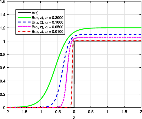
and
with
, and different values of
.
4 Convergence analysis
For a fixed value of the parameter , an optimal control problem on the time horizon is introduced as follows: where presents the feasible region. Suppose that is a decreasing sequence (i.e., ) and satisfies the equality . Further, this leads to a sequence of optimal control problems (i.e., problem (4.1a)-(4.1d) with ). Note that and , are continuous on the compact set U. Thus, is a compact set and problem (4.1a)-(4.1d) can obtain an optimal solution in . In addition, and , are also continuously differentiable functions. Thus, the solution of problem (4.1a)-(4.1d) can be obtained by using any gradient-based numerical optimization algorithm. Now, our main interest is the relation between problems (4.1a)-(4.1d) and (2.1a)-(2.1e).
4.1 Convergence analysis of feasible regions
By using the property (2) of , if follows that , for any . Particularly, the sequence satisfies , for any sequence with . Further, is guaranteed under Assumption 3.1 (see Theorem 3.1). Next, the following Theorem will show that the feasible regions of problem (4.1a)-(4.1d) with are uniformly convergent to the feasible region of problem (2.1a)-(2.1e).
Theorem 4.1. Suppose that
is a sequence satisfying
. Then, Assumption 3.1 indicates that
Proof. Note that is a sequence consisting of compact sets, , the set U is compact, (see Theorem 3.1), and the set is also compact. Then, by using the definition of the Hausdorff distance, we can obtain that This completes the proof of Theorem 4.1.
Remark 4.1. Note that the results of Theorem 3.1 and 4.1 is true for any sequence
with
and
. Then, these results can be summarized as follows:
In generally, it is challenging to obtain the exact analytic representation for the stochastic constraints described by (2.1d). In addition, it is also very difficulty to solve directly problem (2.1a)-(2.1e) numerically on . Fortunately, the above analysis and discussion show that can be as close as possible to and equal to in the limit. This implies that we can obtain the numerical solution of problem (2.1a)-(2.1e) on with .
4.2 Convergence analysis of approximate solutions
From the definition of problem (4.1a)-(4.1d) and the properties (1)-(3) of , it follows that any solution of problem (4.1a)-(4.1d) is a feasible solution of problem (3.6a)-(3.6e). Further, for any , the objective function’s optimal value of problem (4.1a)-(4.1d) is an upper bound for the objective function’s optimal value of problem (2.1a)-(2.1e). Next, the following Theorem will show that any limit point of the local optimal solution sequence of problem (4.1a)-(4.1d) is also a local optimal solution of problem (2.1a)-(2.1e).
Theorem 4.2. Suppose that is a sequence and is a local optimal solution of problem (4.1a)-(4.1d), for any . Then, there exists a subsequence of such that and there exists an open ball around such that and is a local optimal solution of problem (2.1a)-(2.1e). Inversely, if is a strict local optimal solution of problem (2.1a)-(2.1e), then there exists a local optimal solution sequence of problem (4.1a)-(4.1d) such that .
Proof. Note that the set U is compact and . Thus, there exists a subsequence of such that . Since and (see Theorem 3.1), one can obtain that . Further, for a sufficiently large , there exists a ball such that is a local optimal solution of problem (4.1a)-(4.1d).
Suppose that
is not a local optimal solution of problem (2.1a)-(2.1e). This indicates that there exists a
such that
Suppose that is a local optimal solution of problem (2.1a)-(2.1e). Let , for any , where denotes the closure of C and the inequality constraints , hold true, for a bounded ball . Further, let , for any with . By using the compactness of , it follows that there exists a sequence such that . Note that . Thus, by using the continuity of the objective function , it follows that for any with . Thus, . If , then this is in contradiction with is a strict local optimal solution of problem (2.1a)-(2.1e). Thus, the sequence converges to , where is the local optimal solution of problem (4.1a)-(4.1d). This completes the proof of Theorem 4.2.
5 Solving problem (4.1a)-(4.1d)
In generally, it is challenging to obtain an analytical solution of problem (4.1a)-(4.1d). To solve this problem numerically, an important strategy is to discretize the dynamical system such that the original optimal control problem can be transformed into a nonlinear parameter optimization problem with stochastic constraints.
5.1 Time domain transformation
To construct the method of solving problem (4.1a)-(4.1d), the time domain is required to be transformed from
to
by using the following scaling transformation:
5.2 Problem discretization
Numerical computation approaches for optimal control problems can be divided into two categories: indirect approaches and direct approaches. The idea of indirect approaches is that the optimality conditions are established by using variational techniques and the original optimal control problem can be transformed into a Hamiltonian boundary-value problem. Unfortunately, the Hamiltonian boundary-value problem is usually ill-conditioned because of hypersensitivity. The idea of direct approaches is that the control input and/or system state are parameterized by using basis functions and the original optimal control problem can be transformed into a finite-dimensional nonlinear optimization problem. Although direct approaches usually are less ill-conditioning, many existing approaches either are inaccurate or provide no costate information. To overcome this difficulty, the Gaussian quadrature orthogonal collocation approach is developed for solving optimal control problems in recent years. Its idea is that the system state and control input are approximated by using a basis of global polynomials and are discretized at a set of discretization points. In this paper, Legendre–Gauss-Radau points (Kameswaran and Biegler, 2008) are adopted as the discretization points. Suppose that
are M Legendre–Gauss-Radau points, where
and
. To contain the terminal time
, the point
is added to the discretization point set. Now, a basis of Lagrange polynomials are defined as follows:
To solve problem (5.12a)-(5.12e), the Monte Carlo sample method is adopted to compute the expectation value in Eq. (5.12c). Let be samples following the distribution . Then, problem (5.12a)-(5.12e) can be approximated by which is a static nonlinear programming problem and can be solved by using any gradient-based numerical optimization algorithm.
Remark 5.1. The work (Kameswaran and Biegler, 2008) shows that the solution accuracy can be improved by using a larger value of the number M for Legendre–Gauss-Radau points. However, it may greatly increase the computation amount of the numerical computation approach developed by this paper. In order to balance the computation amount and the numerical solution accuracy, Section 6.7 (i.e., Processing power analysis) will propose a sensitivity analysis method to set the value of the parameter M.
5.3 Solving problem (4.1a)-(4.1d)
For simplicity, we suppose that is defined by , where . Based on the above analysis and discussion, the following numerical optimization algorithm is proposed for solving problem (4.1a)-(4.1d).
Algorithm 5.1.
Step 1: Initialize , choose the tolerance , set .
Step 2: Generate M samples following the distribution .
Step 3: Solve problem (5.13a)-(5.13e) by using the sequential quadratic programming method, and suppose that the solution obtained is .
Step 4: If , then stop and go to Step 5. Otherwise, set and , and go to Step 3.
Step 5: Construct the solution of problem (4.1a)-(4.1d) from by using (5.5), and output the corresponding optimal objective function value .
Remark 5.2. This method proposed by this paper is designed for problem (2.1a-2.1e), in which the random variable has an arbitrary probability distribution. Note that any limit point of the local optimal solution sequence of problem (4.1a)-(4.1d) is also a local optimal solution of problem (2.1a)-(2.1e) (see Theorem 4.2). Then, a solution of problem (2.1a)-(2.1e) is also obtained, as long as the parameter is sufficiently small. Thus, Algorithm 5.1 can be used to obtain a solution of problem (2.1a-2.1e), in which the random variable has an arbitrary probability distribution.
6 Numerical results
In this section, the nonlinear continuous stirred-tank reactor problem (Jensen, 1964; Lapidus and Luus, 1967) is further extended to illustrate the effectiveness of the approach developed by Sections 2–5 by introducing some stochastic constraints. All numerical simulation results are obtained under Windows 10 and Intel Core i7-1065G7 CPU, 3.9 GHz, with 8.00-GB RAM.
6.1 Nonlinear continuous stirred-tank reactor
As shown in Fig. 6.1, the nonlinear continuous stirred-tank reactor problem describes several simultaneous chemical reactions taking place in an isothermal nonlinear continuous stirred-tank reactor. The control variables are an electrical energy input used to promote a photochemical reaction and three feed stream flow rates. The objective of this problem is to maximize the economic benefit by choosing the control variables of the nonlinear continuous stirred-tank reactor. This problem can be described by an optimal control problem with stochastic constraints as follows: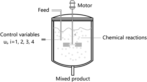
Schematic diagram of a nonlinear continuous stirred-tank reactor..
Choose the control input
over the time horizon
to maximize the objective function
6.2 Parameter description
To discretized the nonlinear continuous-time dynamical system, we adopt
Legendre–Gauss-Radau points. Let
and
. In order to make Algorithm 5.1 converge quickly, we set
, which satisfies the stochastic constraints (6.4)-(6.8) (i.e.,
is an admissible control). Then, the technique proposed in Sections 3 and 4 of this paper is adopted to transform the stochastic constraints describe by (6.4)-(6.7). Based on the analysis and discussion of Sections 3 and 4, these stochastic constraints can be transformed into the following form:
Following the above transformation method, the original nonlinear continuous stirred-tank reactor problem with stochastic constraints is rewritten as a deterministic constrained optimal control problem, which can be solved by using some existing numerical algorithms. In this paper, all the numerical simulation results are obtained by using the technique proposed in Sections 3–5 with the sequential quadratic programming method.
6.3 Impact of the parameter
In this subsection, we will investigate the sensitivity analysis of the parameter
with the proposed numerical computation method. In generally, it is usually difficult to choose a suitable value of the parameter
as the parameter
does not involve any clear physical meaning. Based on Theorem 3.1 described by Section 3 and Theorems 4.1–4.2 described by Section 4, the solution accuracy can be improved by using a larger value of the parameter
. Unfortunately, it may give rise to some computational difficulties for the proposed numerical computation method. By specifying
, the numerical simulation results are presented by Fig. 6.2, which implies that the numerical solution is sensitive with respect to the value of the parameter
. In other words, a better objective value, together with a more aggressive stochastic constraint violation rate, can be obtained by increasing the value of the parameter
. Thus, a suitable treatment of the parameter
is needed. For this reason, an adaptive strategy is designed in Algorithm 5.1.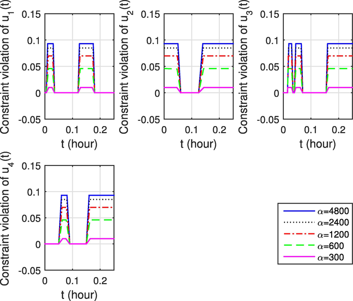
Numerical results of sensitivity analysis with respect to the parameter
.
6.4 Numerical simulation results
The numerical computation method proposed in Sections 3–5 is adopted to solve the nonlinear continuous stirred-tank reactor problem and the corresponding numerical simulation results are presented by Figs. 6.3,6.4. Further, the stochastic constraint violation of the proposed numerical computation method is presented by Fig. 6.5, which shows that all the nonnegative constrains described by (6.8) can be satisfied strictly, whereas the control input cannot achieve its boundary values exactly due to the consideration of stochastic limits. In addition, from Fig. 6.5, the violation rate of stochastic constraints can be smaller than the maximum allowable values
, during the time horizon
. These numerical simulation results imply that the effectiveness of the proposed numerical computation method can be well guaranteed.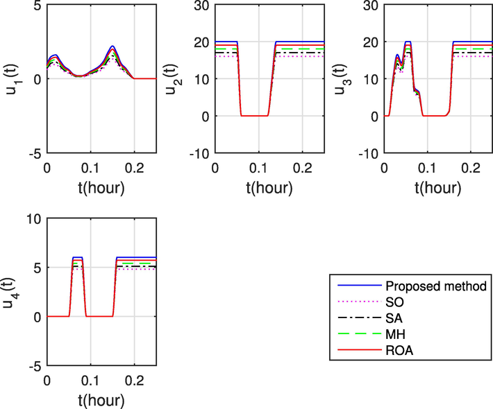
The optimal control input obtained by using the SO approach (Calafiore and Campi, 2006), the SA method (Luedtke and Ahmed, 2008), the MH algorithm (Poojari and Varghese, 2008), the ROA technique (Li and Li, 2015), and the numerical computation method proposed by this paper..
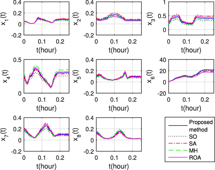
The optimal system state obtained by using the SO approach (Calafiore and Campi, 2006), the SA method (Luedtke and Ahmed, 2008), the MH algorithm (Poojari and Varghese, 2008), the ROA technique (Li and Li, 2015), and the numerical computation method proposed by this paper..
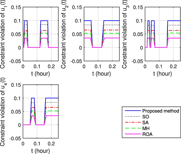
Constraint violations of
, and
obtained by using the SO approach (Calafiore and Campi, 2006), the SA method (Luedtke and Ahmed, 2008), the MH algorithm (Poojari and Varghese, 2008), the ROA technique (Li and Li, 2015), and the numerical computation method proposed by this paper.
6.5 Comparison with other typical approaches
To further illustrate the effectiveness of the proposed numerical computation method, a comparative research is adopted to analyze the optimal system state trajectories and the stochastic constraint violations by implementing the proposed numerical computation method and the other typical approaches. For example, the scenario optimization (SO) approach (Calafiore and Campi, 2006), the sample approximation (SA) method (Luedtke and Ahmed, 2008), the meta-heuristic (MH) algorithm (Poojari and Varghese, 2008), and the robust optimization approximation (ROA) technique (Li and Li, 2015). It should be pointed out that the SO approach and the SA method are two different sampling based methods. In the SO approach, a set of samples are adopted for the stochastic variable so that the stochastic constraints can be approximately replaced by using some deterministic constraints. For the SA method, an empirical distribution obtained from a random sample is used to replace the actual distribution. Further, it can be used to evaluate the stochastic constraints. The MH algorithm is also a sampling based method. In the MH algorithm, the stochastic nature is processed by using the Monte Carlo simulation, whereas the non-convex and nonlinear nature of the optimization problem with stochastic constraints are addressed by using the Genetic Algorithm. Unfortunately, these three methods are designed to obtain feasible solutions without any optimality guarantees. The ROA technique is an analytical approximation method. Its idea is that the stochastic constraint is transformed into a deterministic constraint. Compared with the SO approach, the SA method, and the MH algorithm, it can provide a safe analytical approximation, the size of the corresponding problem is independent of the solution reliability, and needs only a mild assumption on random distributions. However, this safe approximation may lead to the conservatism is very high and the corresponding solution has very poor performance in practice. The optimal system state and control input obtained by using the other typical approaches are also presented by Figs. 6.3 and 6.4 and the corresponding stochastic constraint violation is presented by Fig. 6.5.
Detailed numerical simulation results with relation to the maximum violation rates
, for the stochastic constraints and the optimal value of objective function
for different approaches are presented by Table 6.1. From Figs. 6.3 and 6.5, it follows that the nonnegative constrains and the stochastic constraints can be satisfied by the SO approach, the SA method, the MH algorithm, the ROA technique, and the proposed numerical computation method. Thus, these five approaches are all feasible for solving the nonlinear continuous stirred-tank reactor problem. Further, according to the data or information provided by Table 6.1 and Fig. 6.5, the proposed numerical computation method can usually perform better than the SO approach, the SA method, the MH algorithm, and the ROA technique. More specifically, compared with the SO approach, the SA method, the MH algorithm, and the ROA technique, the constraint violation rates obtained by using the proposed numerical computation method is closer to the maximum violation rates, which implies that it can offer a better solution.
Algorithms
Maximum
Violation
Rate
Objective function value
SO
3.4581%
3.5157%
3.4608%
3.3982%
18.4572
SA
5.3369%
5.2892%
5.3587%
5.2186%
19.3401
MH
6.2983%
6.4753%
6.3242%
6.4995%
19.8322
ROA
8.4675%
8.3696%
8.2678%
8.3702%
20.6925
Proposed method
9.9241%
9.9389%
9.9182%
9.9816%
21.7922
6.6 Stability and robustness analysis
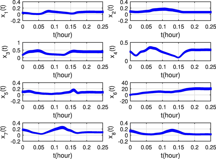
In this subsection, we will present the results of a 1000-trial Monto-Carlo analysis. The main purpose for implementing this analysis is to further illustrate the stability and robustness of the proposed numerical computation method with some small perturbations in initial system state. In every trial, the initial system state is defined by
, where
and
. The numerical simulation results for 600 realizations with some small perturbations in initial system state is presented by Figs. 6.6 and 6.7. From these two figures, it follows that the introduction of some small perturbations in initial system state will give rise to some differences with respect to the optimal system state trajectory. Fortunately, the corresponding violation rates are less than the preassigned risk parameter values. In addition, all numerical simulation results can successfully converge to the neighbourhood of the optimal solution for the nonlinear continuous stirred-tank reactor problem, which indicates that the proposed numerical computation method is stable and robust with respect to the small perturbations in initial system state.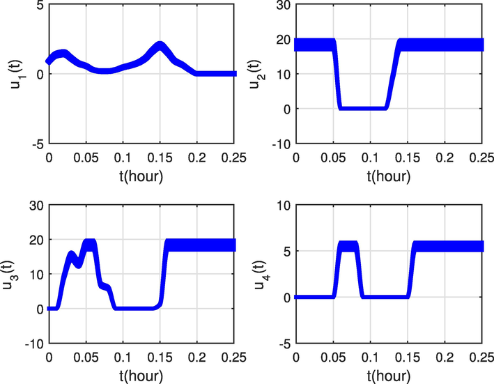
The system state obtained by using the proposed numerical computation method for 1000 realizations with some small perturbations in initial system state.
Violation rates of
, and
obtained by using the proposed numerical computation method for 1000 realizations with some small perturbations in initial system state.
6.7 Processing power analysis
In this subsection, we will investigate and analyze the processing power of the proposed numerical computation method. The total calculated cost of the proposed approach is mainly depended on the following two aspects: one is the function evaluations, the other is the time needed for the calculation of the nonlinear programming solver. If M Legendre–Gauss-Radau points are used, then the numbers of decision variables and the function evaluations become
and
, respectively. Clearly, the nonlinear programming solver requires more computation than the function evaluation part. In addition, the computational process is sensitive with respect to the tolerance
described by Algorithm 5.1. A sensitivity analysis for the tolerance
is implemented and the numerical simulation results are presented by Table 6.2. From Table 6.2, it follows that the computation time for the nonlinear continuous stirred-tank reactor problem is monotonically increasing as the tolerance
becomes smaller. In order to balance the computation amount and the numerical solution accuracy, the tolerance
is set to
in this paper.
Values for the tolerance
Objective function value
17.0541
19.7640
20.3690
21.7922
21.8327
21.8401
CPU time (second)
0.6480
0.6529
0.6703
5.2775
8.3590
19.3240
Although the solution accuracy can be improved by using a larger value of the number M for Legendre–Gauss-Radau, it may greatly increase the computation amount of the numerical computation approach developed by this paper. Note that the computational process is also sensitive with respect to the the parameter M. Then, a sensitivity analysis for the parameter M is implemented and the numerical simulation results are presented by Table 6.3. From Table 6.3, it follows that the computation time for the nonlinear continuous stirred-tank reactor problem is monotonically increasing as the parameter M becomes larger. In order to balance the computation amount and the numerical solution accuracy, the parameter M is set to
in this paper.
Values for the parameter M
Objective function value
15.8483
18.9181
19.5481
21.7922
21.8346
21.8412
CPU time (second)
0.6022
0.6263
0.6419
5.2775
8.3621
19.3323
In conclusion, above numerical simulation results show that compared with compared with the SO approach, the SA method, the MH algorithm, and the ROA technique, the proposed numerical computation method is less conservative and can obtain a stable and robust performance when considering the small perturbations in initial system state.
7 Conclusion
In this paper, a convergent approximation approach is proposed and used for solving the optimal control problem for nonlinear chemical processes with stochastic constraints. The main feature of this approach is that it introduces a smooth and differentiable function to obtain a subset of feasible solutions of the stochastic-constrained optimal control problem. Further, the convergence analysis results show that the approximation function and the corresponding feasible set converge uniformly to that of the original optimal control problem as the adjusting parameter reduces. Following that, a numerical computation approach is proposed for solving the original optimal control problem. Finally, in order to verify the effectiveness of the approach proposed by this paper, the nonlinear continuous stirred-tank reactor problem is extended by considering some stochastic constraints. Subsequently, the proposed approach is used to solve this stochastic-constrained optimal control problem. The numerical simulation results and the comparative study show that compared with other existing typical methods, the proposed approach is less conservative and can obtain a stable and robust performance when considering the small perturbations in initial system state.
Acknowledgements
The authors express their sincere gratitude to Professor Abdulrahman Abdullah Alwarthan, the editor, and the anonymous reviewers for their constructive comments in improving the presentation and quality of this manuscript. This work was supposed by the National Natural Science Foundation of China under Grant Nos. 61963010 and 61563011, and the Special Project for Cultivation of New Academic Talent and Innovation Exploration of Guizhou Normal University, PR China in 2019 under Grant No. 11904-0520077.
Declaration of Competing Interest
The authors declare that they have no known competing financial interests or personal relationships that could have appeared to influence the work reported in this paper.
References
- Development of multiple machine-learning computational techniques for optimization of heterogenous catalytic biodiesel production from waste vegetable oil. Arabian J. Chem.. 2022;15:103843.
- [Google Scholar]
- Optimal control and the Pontryagin’s principle in chemical engineering: History, theory, and challenges. AIChE J. 2022
- [CrossRef] [Google Scholar]
- Optimality-based grid adaptation for input-affine optimal control problems. Comput. Chem. Eng.. 2016;92:189-203.
- [Google Scholar]
- A simple proof of the discrete time geometric Pontryagin maximum principle on smooth manifolds. Automatica 2020
- [CrossRef] [Google Scholar]
- Adaptive dynamic programming and optimal control of nonlinear nonaffine systems. Automatica. 2014;50:2624-2632.
- [Google Scholar]
- Dynamic optimization in the design and scheduling of multiproduct batch plants. Ind. Eng. Chem. Res.. 1996;35:2234-2246.
- [Google Scholar]
- Modeling chemical process systems via neural computation. IEEE Control Syst. Mag.. 1990;10:24-30.
- [Google Scholar]
- Pontryagin maximum principle for finite dimensional nonlinear optimal control problems on time scales. SIAM J. Control Optim.. 2013;51:3781-3813.
- [Google Scholar]
- Output feedback stochastic nonlinear model predictive control for batch processes. Comput. Chem. Eng.. 2019;126:434-450.
- [Google Scholar]
- The scenario approach to robust control design. IEEE Trans. Auto. Control. 2006;51:742-753.
- [Google Scholar]
- Direct and indirect optimal control applied to plant virus propagation with seasonality and delays. J. Comput. Appl. Math. 2020
- [CrossRef] [Google Scholar]
- Dynamic optimization of nonlinear processes by combining neural net model with UDMC. Aiche J.. 1994;40:1488-1497.
- [Google Scholar]
- A bilevel NLP sensitivity-based decomposition for dynamic optimization with moving finite elements. AIChE J.. 2014;60:966-979.
- [Google Scholar]
- Constrained linear quadratic optimal control of chemical processes. Comput. Chem. Eng.. 2000;24:823-827.
- [Google Scholar]
- Direct and indirect methods in optimal control with state constraints and the climbing trajectory of an aircraft. Optim. Control Appl. Meth.. 2018;39:281-301.
- [Google Scholar]
- Parameter estimation and optimal control of a batch transesterification reactor: An experimental study. Chem. Eng. Res. Design. 2020;157:1-12.
- [Google Scholar]
- Robust and Optimal Control. New Jersey: Prentice Hall; 1995.
- Integrating robustness, optimality and constraints in control of nonlinear processes. Chem. Eng. Sci.. 2001;56:1841-1868.
- [Google Scholar]
- Dispatching-like strategies using intermediate storage for the scheduling of batch chemical processes. Comput. Chem. Eng.. 1995;19:621-626.
- [Google Scholar]
- Optimal feedback control of batch self-assembly processes using dynamic programming. J. Process Control. 2020;88:32-42.
- [Google Scholar]
- A hierarchical decision procedure for productivity innovation in large-scale petrochemical processes. Comput. Chem. Eng.. 2008;32:1029-1041.
- [Google Scholar]
- How to verify optimal controls computed by direct shooting methods?-A tutorial. J. Process Control. 2012;22:494-507.
- [Google Scholar]
- Jensen, T., 1964. Dynamic control of large dimension nonlinear chemical processes, Ph.D. Dissertation, Princeton University.
- Convergence rates for direct transcription of optimal control problems using collocation at Radau points. Comput. Optim. Appl.. 2008;41:81-126.
- [Google Scholar]
- Event triggered control for fault tolerant control system with actuator failure and randomly occurring parameter uncertainty. Appl. Math. Comput.. 2022;415:126714.
- [Google Scholar]
- A direct transcription-based multiple shooting formulation for dynamic optimization. Comput. Chem. Eng. 2020
- [CrossRef] [Google Scholar]
- Optimal control of hybrid electric vehicles based on Pontryagin’s minimum Principle. IEEE Trans. Control Syst. Tech.. 2011;19:1279-1287.
- [Google Scholar]
- A dynamic optimization framework for integration of design, control and scheduling of multi-product chemical processes under disturbance and uncertainty. Comput. Chem. Eng.. 2017;106:147-159.
- [Google Scholar]
- Optimal control of engineering processes. Waltham, MA: Blaisdell; 1967.
- Optimization and design of machine learning computational technique for prediction of physical separation process. Arabian J. Chem.. 2022;15:103680.
- [Google Scholar]
- Robust distributed model predictive control of constrained continuous-time nonlinear systems: A robustness constraint approach. IEEE Trans. Auto. Control. 2013;59:1673-1678.
- [Google Scholar]
- Optimal robust optimization approximation for chance constrained optimization problem. Comput. Chem. Eng.. 2015;74:89-99.
- [Google Scholar]
- A multi-objective robust optimization scheme for reducing optimization performance deterioration caused by fluctuation of decision parameters in chemical processes. Comput. Chem. Eng.. 2018;119:1-12.
- [Google Scholar]
- A sample approximation approach for optimization with probabilistic constraints. SIAM J. Optim.. 2008;19:674-699.
- [Google Scholar]
- Operational design for start-up of chemical processes. Comput. Chem. Eng.. 1997;21:997-1007.
- [Google Scholar]
- Optimization of chemical processes with dependent uncertain parameters. Chem. Eng. Sci.. 2012;83:119-127.
- [Google Scholar]
- Optimal design of chemical processes with chance constraints. Comput. Chem. Eng.. 2013;59:74-88.
- [Google Scholar]
- Optimal Bayesian experiment design for nonlinear dynamic systems with chance constraints. J. Process Control. 2019;77:155-171.
- [Google Scholar]
- Deterministic approximations of probability inequalities. Math. Meth. Oper. Res.. 1989;33:219-239.
- [Google Scholar]
- Genetic algorithm based technique for solving chance constrained problems. Eur. J. Oper. Res.. 2008;185:1128-1154.
- [Google Scholar]
- Stochastic back-off approach for integration of design and control under uncertainty. Ind. Eng. Chem. Res.. 2018;57:4351-4365.
- [Google Scholar]
- A review of pseudospectral optimal control: From theory to flight. Annu. Rev. Control. 2012;36:182-197.
- [Google Scholar]
- Approximate convex hull based scenario truncation for chance constrained trajectory optimization. Automatica. 2020;112:108702.
- [Google Scholar]
- Active robust optimization: Enhancing robustness to uncertain environments. IEEE Trans. Cybern.. 2014;44:2221-2231.
- [Google Scholar]
- Optimization of structural and operational variables for the energy efficiency of a divided wall distillation column. Comput. Chem. Eng.. 2012;40:33-40.
- [Google Scholar]
- Control structure design for complete chemical plants. Comput. Chem. Eng.. 2004;28:219-234.
- [Google Scholar]
- Simultaneous design & control of a reactive distillation system-A parametric optimization & control approach. Chem. Eng. Sci. 2021
- [CrossRef] [Google Scholar]
- A survey of optimal process design capabilities and practices in the chemical and petrochemical industries. Comput. Chem. Eng.. 2018;112:180-189.
- [Google Scholar]
- Data-driven adaptive probabilistic robust optimization using information granulation. IEEE Trans. Cybern.. 2016;48:450-462.
- [Google Scholar]
- Analysis of the stability and controllability of chemical processes. Comput. Chem. Eng.. 2011;35:1101-1109.
- [Google Scholar]
- Hybrid stochastic optimization method for optimal control problems of chemical processes. Chem. Eng. Res. Design. 2017;126:297-310.
- [Google Scholar]
- Optimal control of constrained switched systems and application to electrical vehicle energy management. Nonlinear Anal. Hybrid Syst.. 2018;30:171-188.
- [Google Scholar]
- Numerical algorithm for optimal control of switched systems and its application in cancer chemotherapy. Appl. Soft Comput.. 2022;115:108090.
- [Google Scholar]
- Switched system optimal control approach for drug administration in cancer chemotherapy. Biomed. Signal Process. Control. 2022;75:103575.
- [Google Scholar]
- Chance constrained dynamic optimization approach for single machine scheduling involving flexible maintenance, production, and uncertainty. Eng Appl Artif. Intel.. 2022;114:105024.
- [Google Scholar]
- Passenger evacuation path Planning in subway station under multiple fires based on multiobjective robust optimization. In: IEEE Trans. Intell. Transport. Syst.. 2022.
- [CrossRef] [Google Scholar]
- Model-free vibration control based on a virtual controlled object considering actuator uncertainty. J. Vib. Control. 2021;27:1324-1335.
- [Google Scholar]
- Optimal control for nonlinear continuous systems by adaptive dynamic programming based on fuzzy basis functions. Appl. Math. Model.. 2016;40:6766-6774.
- [Google Scholar]
- Near-optimal control of nonlinear dynamical systems: A brief survey. Annu. Rev. Control. 2019;47:71-80.
- [Google Scholar]
- Asynchronous nonfragile guaranteed cost control for impulsive switched fuzzy systems with quantizations and its applications. IEEE Trans. Fuzzy Syst. 2022
- [CrossRef] [Google Scholar]


