

Translate this page into:
Optimization and design of machine learning computational technique for prediction of physical separation process
⁎Corresponding authors. proudchina2008@163.com (Haiqing Li), lotfor@ums.edu.my (Md Lutfor Rahman)
-
Received: ,
Accepted: ,
This article was originally published by Elsevier and was migrated to Scientific Scholar after the change of Publisher.
Peer review under responsibility of King Saud University.
Abstract
Machine learning (ML) methods were developed and optimized for description and understanding a physical separation process. Indeed, this work indicates application of machine learning technique for a real physical system and optimization of process parameters to achieve the target. A bunch of datasets were extracted from resources for physical adsorption process in removal of impurities from water as a case study to test the developed machine learning model. The case study process is adsorption process which has extensive application in science and engineering. The machine learning (ML) method was developed, and the parameters were optimized in order to get the best simulation’s performance for adsorption process. The data are used to correlate the adsorption capacity of the material to the adsorption parameters including dosage and solution pH. Randomized training and validation were performed to predict the process’s output, and great agreement was obtained between the predicted values and the observed values with R2 values greater than 0.9 for all cases of training and validation at the optimum conditions. Three different machine learning techniques including Random Forest (RF), Extra Tree (ET), and Gradient Boosting (GB) were employed for the adsorption data. Quantitatively, R2 scores of 0.958, 0.998, and 0.999 were obtained for RF, GB, and ET, respectively. It was indicated that GB and ET models performed almost the same and better than RF in prediction of adsorption data.
Keywords
Machine learning
Artificial intelligence
Modeling
Optimization
Separation

1 Introduction
Separation of a target component from a liquid mixture has extensive applications in science and engineering, for instance in chemical and biochemical industries. The target component is usually removed due to certain reasons. It could be either the unwanted component which must be removed from the solution, or the desire component for purification purposes (Chen, 2021a, 2021c, 2021d; Ghodke, 2020; Hasthavaram, 2020; Hu, 2021; Li, 2021; Qaderi, 2020; Shang, 2022; Yang, 2021). The purification can be performed on feed/raw materials or the final products in manufacturing industries. The separation is mainly governed by mass transfer which depends on the gradients of properties in the system such as concentration gradient (Aroon et al., 2020; Dong et al., 2021; Elgersma, 2022; Kumar Chaurasiya and Singh, 2021; Shirazian and Ashrafizadeh, 2011; Shirazian et al., 2009, 2012; Sohrabi, 2011). Basically, the rate of mass transfer for the target component determines the separation efficiency and performance of the unit operation used for separation (Ghadiri and Shirazian, 2013; Ghadiri et al., 2012; Marjani and Shirazian, 2012; Pishnamazi, 2020; Ranjbar, 2013; Riasat Harami, 2019; Shirazian and Ashrafizadeh, 2010, 2010, 2013, 2015; Shirazian, 2012, 2012). Indeed, improving the mass transfer is the key step in development of separation processes.
Separation can be conducted in different unit operations such as distillation, absorption, adsorption, membrane processes, etc. Depending on the degree of separation as well as the energy requirements, appropriate separation process can be selected and used for separation of target components. When the amount of target component concentration in the liquid phase is low, then adsorption is an attractive unit operation for the separation of target molecules from liquid mixture (Albadarin, 2017; Chachkov and Mikhailov, 2020; Chen, 2021b; Chupradit, 2021; Fatima et al., 2020; Khansary et al., 2017; Mengting, 2019; Shirazian and Ashrafizadeh, 2015; Shtamburg, 2020; Soltani et al., 2020; Soltani, 2020). This separation technique is based on selective removal of the target component from a mixture. Therefore, the affinity between the adsorbent and the target molecule is the key step in the adsorption process (Albadarin, 2017; Ghadiri, 2013; Mengting, 2019; Razavi et al., 2015; Rezakazemi and Shirazian, 2019; Shirazian and Ashrafizadeh, 2015; Soltani et al., 2020; Soltani, 2020, 2020). The design of the adsorbent should be carried out in a way to maximize its separation capacity for separation of the target molecules which can be achieved by enhancing the internal and external surface area of the adsorbent (Asadollahzadeh, 2018; Ghadiri et al., 2014; Harami, 2021; Hasanizadeh et al., 2018; Hemmati, 2015; Khansary et al., 2017; Nerlikar, 2020; Shirazian and Ashrafizadeh, 2015; Soltani et al., 2019; Soltani, 2019, 2020).
By development of computational technique, one can predict the adsorption capacity of a solid material for application in adsorption process. This computational task can be conducted by using different modeling approaches such as machine learning (ML) models which are suitable for fitting large datasets (Ding, 2020; Sajjia, 2017; Senthil et al., 2020; Singh, 2021; Tao, 2021; Wu, 2021; Zhang, 2021; Zhu et al., 2021). However, some machine learning models have been developed for small datasets (Babanezhad, 2020; Ismail, 2019, 2019, 2020; Liang, 2020; Shang, 2021). These models rely on training a dataset and fitting the model to the obtained data. Therefore, measured data are required to train the network (Cai, 2020; Chao, 2019; Meng, 2021; Wang et al., 2022; Wu, 2021; Yang, 2021; Zhang, 2021; Zhao, 2021; Zheng, 2021; Zhou, 2018). This method has been recently used in separation applications based on adsorption process to predict the performance of an adsorbent in removal of impurities from water (González, 2020; Syah, 2021a, 2021b).
In this study, we implemented three different machine learning models for simulation of adsorption data. Indeed, the adsorption capacity of a composite material was predicted at different conditions using the developed models. Indeed, we deal with a regression problem with a very small number of data points which are the adsorption isotherms for a particular adsorbent. In such cases, we can use ensemble methods to build high-generality models. Ensembles, especially ensembles of tree-based models, are one of the most flexible and useful machine learning techniques. An ensemble is a collection of trained models with the goal of improving the predictive performance of a single model by combining their predictions. There are several methods in this class of machine learning algorithms, the most important and famous of which are bagging and boosting (Ding, 2021; Yin, 2021, 2021).
Bagging (short for “bootstrap aggregating”) approaches fit several considered learners independently of others, allowing them to be trained concurrently. The goal of this strategy is to create an ensemble model that is more robust than the individual models that comprise it.
In boosting at first, a subset is selected, and all data points are assigned equal weights. On this subset, a foundation model is built. This model is used to forecast the entire dataset. Errors are then determined using the actual and anticipated values. Higher weights are assigned to data that were mistakenly anticipated. A new model is built, and predictions are made on the dataset. Similarly, many models are developed, each one correcting the preceding model's flaws. The weighted mean of all the models is used to create the final model (strong learner).
Fig. 1 shows the difference between the bagging and boosting methods schematically. Based on these facts and figures, in this research, we have selected three different models consisting of two bagging models and a boosting model. In the following, we will discuss these methods and their results on the dataset of this research. These models include Random Forest (bagging), Gradient Boosting, and Extra Tree (boosting).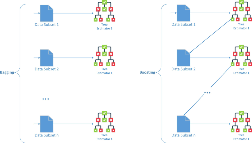
Bagging vs. Boosting ensembles.
2 Dataset used
The dataset used in this study is similar (Soltani, 2021) which is taken from the literature (Cook, 1977). More information on how to collect this data set can be found in these two references. This dataset has 21 data points, which are shown in full in Table 1. In this regression problem, we have two inputs: adsorbent dosage [W(g] and solution pH, the first of which is floating point decimal number and the second of which is positive integer.
W (g)
pH
Qe
0.05
3
15
0.05
4
28.83333
0.05
5
33.75
0.05
6
39.91667
0.05
7
39.41667
0.05
8
38.75
0.05
9
33.16667
0.03
3
10.83333
0.03
4
25
0.03
5
30.83333
0.03
6
37.41667
0.03
7
35.83333
0.03
8
33.33333
0.03
9
28.33333
0.01
3
7.5
0.01
4
21.66667
0.01
5
28.33333
0.01
6
35.5
0.01
7
33.75
0.01
8
28.33333
0.01
9
23.75
The relationship between the inputs as well as the output is shown in Fig. 2 as scatter plot matrix, which shows that there is no definite and linear relationship between these parameters.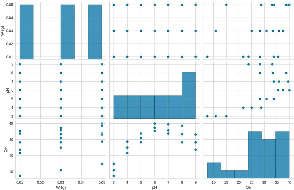
Dataset scatter plot matrix.
3 Methodology
As mentioned before, 3 different models of bagging and boosting have been selected for modeling of the adsorption capacity of the adsorbent in this research. A simple framework shown in Fig. 3 is used to implement the exact models.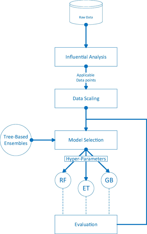
General architecture of the simulation method.
3.1 Preprocessing
Some of the steps shown in Fig. 3 are preprocessors that are needed to prepare the data for better modeling, including influential analysis and scaling. In order to carry out the influential analysis in this research, we have used the Cook's distance (Breiman, 2001). The latter has been done in order to find the influence of each data point on final model, and also for scaling we used standard scaling. The Standard Scaler scales data inside each feature so that the distribution is centered around 0 with a standard deviation of 1. Each feature is separately centered and scaled by computing the necessary statistics on the samples in the training set. If the data is not evenly distributed, this is not the best Scaler to utilize.
3.2 Random forest (RF) and extra tree (ET)
Random forest (RF) (Flach, 2012) is a bagging ensemble that attempts to average multiple noisy(weak), but fairly unbiased trees in order to reduce variance. When building a decision tree, RF first selects a set of features at random, and then continues the process of selecting the normal branch within the feature set.
Bootstrap aggregation (bagging) is the foundation of random forests. Instead of creating a single model, the approach generates a series of bootstrap samples, which are random subsets of the dataset generated with replacement. Each model will be unique because each sample is unique. As a result, rather than a regressor that is overfit to the training set, a robust regressor is produced. The algorithm then creates a model ensemble. The ensemble in a simple decision-tree model consists of decision trees that loop through all variables and split the sample based on the best variable at a time, as shown in the pseudocode in Algorithm 1 below.
Algorithm 1. select feature to split
Input: data D, feature list F.
Output: feature f to split on.
For each
:
Split D into subsets D1,…,DL according to value of vj of f:
If
D1
DL
then:
D1
DL
End
End
Output: fbest
The random-forest model extends the decision-tree by employing a technique known as subspace sampling. The random forest splits depend on only a subset of the independent features at a time. By pushing differences between the models, this adds more variety to the ensemble. Additionally, especially in higher dimensional training sets, this step reduces computational cost.
In pseudocode, Algorithm 2 depicts the random forest ensemble creation algorithm.
Algorithm 2. train an ensemble of models from bootstrap samples
Input: data points D, ensemble size T, learning algorithm A.
Output: ensemble of the developed models.
For t = 0 to t = T:
create a bootstrap sample Dt from D by sampling |D| values with exchange.
choose d features.
train a tree network Mt on Dt with no pruning;
Finish
Output:
Assume the training sets are made up of , where is an instance and is the true label.
The significance of a feature f per tree t is computed as follows (Geurts et al., 2006):
For a random forest regression algorithm, there are several parameters to tune. Our random forest regression model's optimization method includes the following parameters:
-
Number of estimators
-
Maximum depth in each tree
Extra trees (Alswaina and Elleithy, 2018) (Extremely randomized trees) is other tree-based ensemble method similar to Random Forest. The ET is a recursively trained ensemble of Decision Trees, and the final model was produced using a big Decision Tree. Each one constructs the tree using the complete dataset, and the appropriate cut point for each split must be determined based on information gain (Xia, 2015). The ET model has two important innovations:
-
the nodes are divided randomly using the cut-point (Lin et al., 2012).
-
the whole training dataset was utilized to build the DT rather than the replica generation using the Bootstrap for other decision tree models, for the random forest model.
3.3 Gradient boosting (GB)
Instead of generating a single optimized model, Gradient Boosting (GB) improves the standard decision tree models using a statistical technique called boosting, whose main idea is to aggregate a series of weak or base models to generate a single strong consensus model (Bühlmann and Yu, 2003; Elith et al., 2008; Yang, 2020). Gradient boosting algorithm in shown in Algorithm 3.
Algorithm 3. gradient boosting algorithm
Input: Training set
, loss function
, number of iterations M.
Output: The final regression function
Initialize:
For m = 1 to M:
End
Output:
And gets:
The gradient boosting framework supports a variety of smooth loss functions, including AdaBoost, LogitBoost, and L2Boosting (Hamilton et al., 2015). For the regression issue, the squared loss function is utilized because of its simplicity and coherence:
3.4 Performance metrics
This study uses three metrics to assess each algorithm's performance:
-
R Squared (R2) is the percentage of the overall variance in the dependent variable that is accounted for by the independent variable [99]:
-
Mean Squared Error (MSE) is an estimator that assesses average squared errors:
-
Rooted MSE (RMSE):
In these equations are observed and are predicted values.
4 Results and discussion
The three models were implemented using the data listed in Table 1 in order to predict the adsorption data. To get the results, we first need to do the pre-processing steps. Fig. 4 shows the Cook distance diagram in the dataset used. According to this diagram, only one of the data points has an excessive effect on the final model. Therefore, this special point is removed from the learning stage.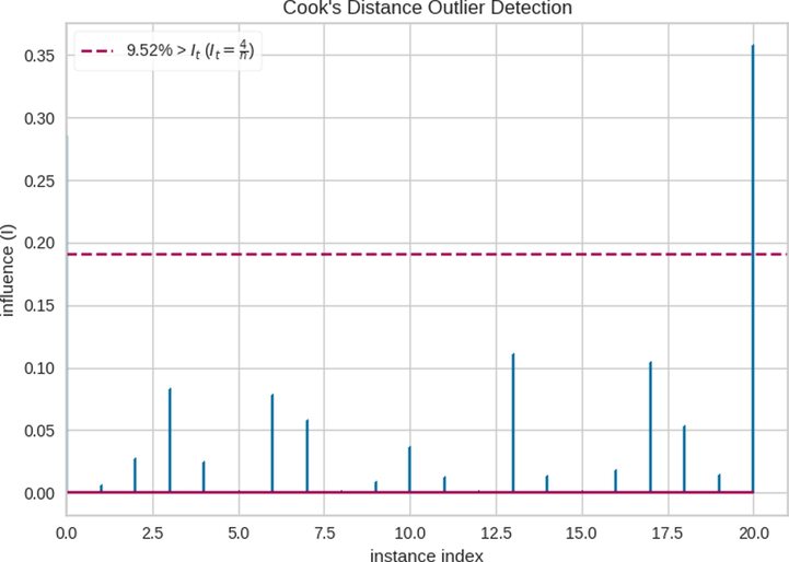
Cooks Distance of Dataset.
To tune the hyperparameters of each of the models introduced in this study, different combinations of the values of these parameters were tested. Finally, we selected the set of values shown in Table 2 as the final values of these parameters.
Hyper-Parameter
Random Forest
Extra Tree
Gradient Boosting
Number of Base Estimators
39
15
45
Maximum Tree Depth
13
6
2
Learning Rate
–
–
0.2
Criterion
Friedman_mse
MAE
–
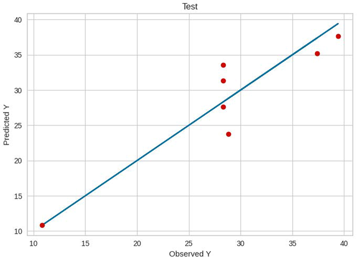
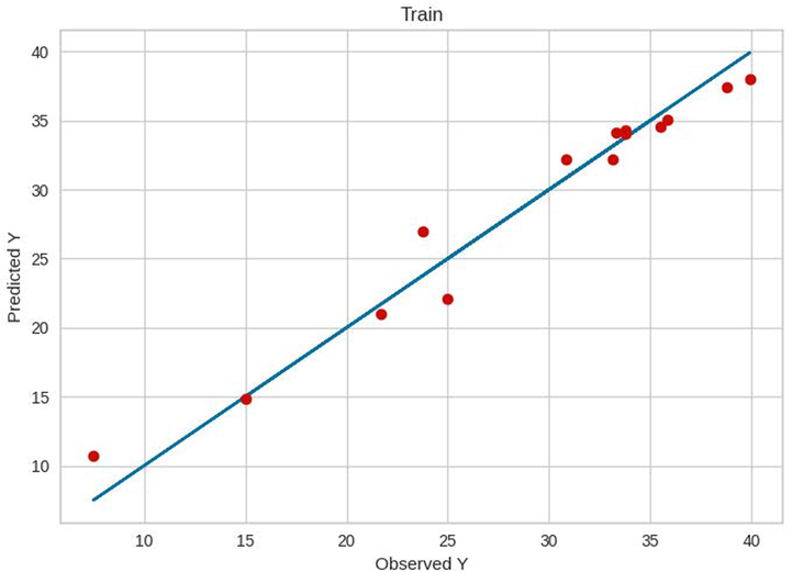
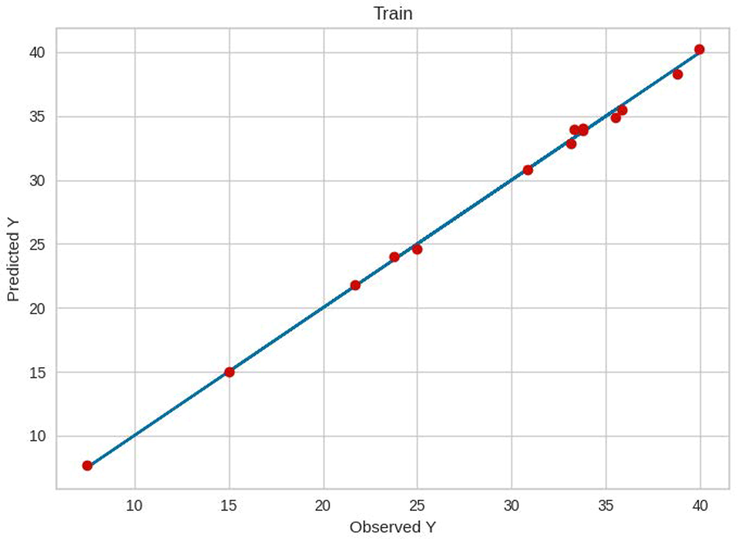
Finally, these parameters were used for the final models, the results of which are shown in Table 3. The results of the residuals for the three models are indicated in Figs. 5–7. Furthermore, the comparisons between the predicted and measured values for the three models are indicated in Figs. 8–13. Based on these results, the ET model can be considered as the best model among these bagging and boosting algorithms. However, the performance of the ET and GB model are almost the same in terms of accuracy as listed in Table 3.
Metric
Random Forest
Extra Tree
Gradient Boosting
R2 score
0.958
0.999
0.998
MSE
9.98
5.40
3.70
RMSE
3.15
2.33
1.92
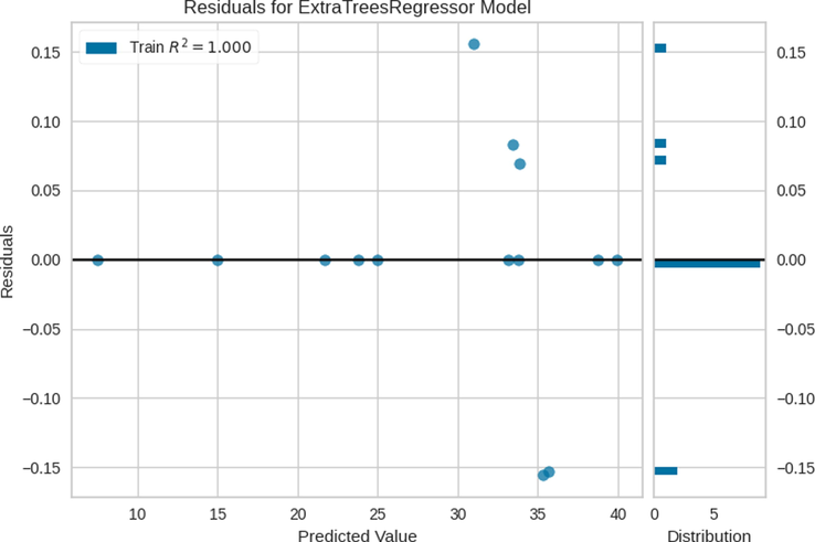
Residuals for ET Model.
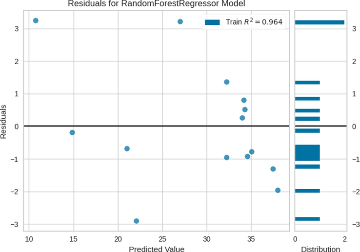
Residuals for RF Model.
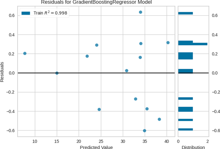
Residuals for GB Model.
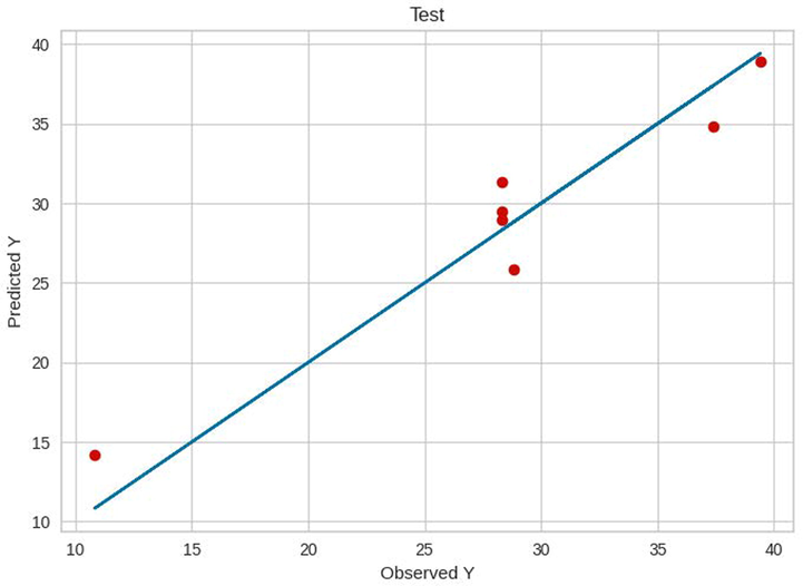
Test results of ET.
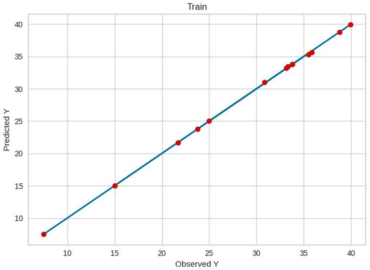
Train results of ET.
Test results of RF.
Train results of RF.
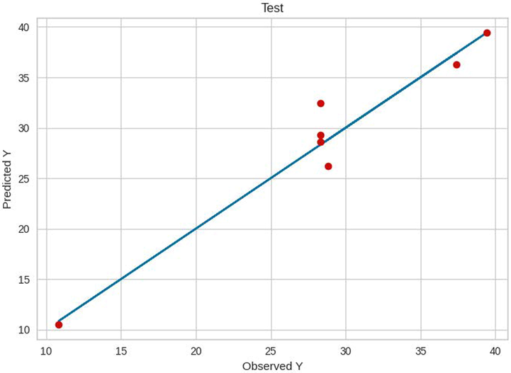
Test results of GB.
Train results of GB.
5 Conclusion
In this study, due to the fact that we were faced with a very small data set, we decided to use bagging and boosting methods for prediction of adsorption capacity of an adsorbent in removal of impurity from water in adsorption process. We considered adsorbent dosage and solution pH as the model inputs, whereas the adsorption capacity was the only predicted output for the models. Three different machine learning models including RF, ET, and GB were considered in this study. Due to the nature of their algorithms, these methods can create highly generalized models in such situations. Fortunately, this hypothesis was confirmed in the practical results of the research. Finally, with R2 criteria, scores of 0.958, 0.998, and 0.999 were obtained for RF, GB, and ET, respectively which is a good result. Also, due to the fact that the selected models are kept as simple as possible, there is the least possibility of over-fitting in them. As a result, we can introduce the ET model as the best predictor of this research. In future research, more parameters can be optimized, and the results can be examined and discussed.
Declaration of Competing Interest
The authors declare that they have no known competing financial interests or personal relationships that could have appeared to influence the work reported in this paper.
References
- Activated lignin-chitosan extruded blends for efficient adsorption of methylene blue. Chem. Eng. J.. 2017;307:264-272.
- [Google Scholar]
- Android malware permission-based multi-class classification using extremely randomized trees. IEEE Access. 2018;6:76217-76227.
- [Google Scholar]
- Revisiting ‘penetration depth’ in falling film mass transfer. Chem. Eng. Res. Des.. 2020;155:18-21.
- [Google Scholar]
- Simulation of Nonporous Polymeric Membranes Using CFD for Bioethanol Purification. Macromol. Theory Simul.. 2018;27(3)
- [Google Scholar]
- Pattern recognition of the fluid flow in a 3D domain by combination of Lattice Boltzmann and ANFIS methods. Sci. Rep.. 2020;10(1):1-13.
- [Google Scholar]
- Boosting with the L 2 loss: regression and classification. J. Am. Stat. Assoc.. 2003;98(462):324-339.
- [Google Scholar]
- Ship Electronic Information Identification Technology Based on Machine Learning. J. Coast. Res.. 2020;103(sp1):770-774.
- [Google Scholar]
- Novel modifications of elemental nitrogen and their molecular structures – a quantumchemical calculation. Eur. Chem. Bull.. 2020;9:78.
- [Google Scholar]
- Using multi-satellite microwave remote sensing observations for retrieval of daily surface soil moisture across China. Water Sci. Eng.. 2019;12:85-97.
- [Google Scholar]
- Enhanced removal of Co(II) and Ni(II) from high-salinity aqueous solution using reductive self-assembly of three-dimensional magnetic fungal hyphal/graphene oxide nanofibers. Sci. Total Environ.. 2021;756:143871
- [Google Scholar]
- Combustion process of nanofluids consisting of oxygen molecules and aluminum nanoparticles in a copper nanochannel using molecular dynamics simulation. Case Stud. Therm. Eng.. 2021;28:101628
- [Google Scholar]
- Facile synthesis of a sandwiched Ti3C2Tx MXene/nZVI/fungal hypha nanofiber hybrid membrane for enhanced removal of Be(II) from Be(NH2)2 complexing solutions. Chem. Eng. J.. 2021;421:129682
- [Google Scholar]
- Engineering of Novel Fe-Based Bulk Metallic Glasses Using a Machine Learning-Based Approach. Arabian J. Sci. Eng.. 2021;46(12):12417-12425.
- [Google Scholar]
- Use of Organic and Copper-Based Nanoparticles on the Turbulator Installment in a Shell Tube Heat Exchanger: A CFD-Based Simulation Approach by Using Nanofluids. J. Nanomater.. 2021;2021:3250058.
- [Google Scholar]
- Detection of influential observation in linear regression. Technometrics. 1977;19(1):15-18.
- [Google Scholar]
- Definition and Application of Variable Resistance Coefficient for Wheeled Mobile Robots on Deformable Terrain. IEEE Trans. Rob.. 2020;36(3):894-909.
- [Google Scholar]
- Artificial intelligence based simulation of Cd (II) adsorption separation from aqueous media using a nanocomposite structure. J. Mol. Liq. 2021117772
- [Google Scholar]
- Gas–liquid mass transfer in the gas–liquid–solid mini fluidized beds. Particuology 2021
- [Google Scholar]
- Measuring the liquid-solid mass transfer coefficient in packed beds using T2–T2 relaxation exchange NMR. Chem. Eng. Sci.. 2022;248:117229
- [Google Scholar]
- Kinetic Study of Fe(II) AND Fe(III) complexes of dopamine, (-)3-(3,4-Dihydroxyphenyl)-L-alanine at physiological pH. Eur. Chem. Bull.. 2020;9:119.
- [Google Scholar]
- Machine learning: the art and science of algorithms that make sense of data. Cambridge University Press; 2012.
- Computational Simulation for Transport of Priority Organic Pollutants through Nanoporous Membranes. Chem. Eng. Technol.. 2013;36(3):507-512.
- [Google Scholar]
- Mass Transfer Simulation of Gold Extraction in Membrane Extractors. Chem. Eng. Technol.. 2012;35(12):2177-2182.
- [Google Scholar]
- Modeling of water transport through nanopores of membranes in direct-contact membrane distillation process. Polym. Eng. Sci.. 2014;54(3):660-666.
- [Google Scholar]
- Computational simulation of mass transfer in extraction of alkali metals by means of nanoporous membrane extractors. Chem. Eng. Process. Process Intensif.. 2013;69:57-62.
- [Google Scholar]
- One-pot synthesis of pyrano[2,3-c]pyrazoles using lemon peel powder as a green and natural catalyst. Eur. Chem. Bull.. 2020;9:38.
- [Google Scholar]
- A practical tutorial on bagging and boosting based ensembles for machine learning: Algorithms, software tools, performance study, practical perspectives and opportunities. Information Fusion. 2020;64:205-237.
- [Google Scholar]
- Relevance of airborne lidar and multispectral image data for urban scene classification using Random Forests. ISPRS J. Photogramm. Remote Sens.. 2011;66(1):56-66.
- [Google Scholar]
- Interpreting regression models in clinical outcome studies. The British Editorial Society of Bone and Joint Surgery London; 2015.
- Mixed Matrix Membranes for Sustainable Electrical Energy-Saving Applications. ChemBioEng Rev.. 2021;8(1):27-43.
- [Google Scholar]
- A novel method for calculating partition coefficient of saline water in direct contact membrane distillation: CFD simulation. Desalin. Water Treat.. 2018;129:24-33.
- [Google Scholar]
- One-pot synthesis of phthalazinyl-2-carbonitrile indole derivatives via [bmim][oh] as ionic liquid and their anti cancer evaluation and molecular modeling studies. Eur. Chem. Bull.. 2020;9:154.
- [Google Scholar]
- Phenol removal from wastewater by means of nanoporous membrane contactors. J. Ind. Eng. Chem.. 2015;21:1410-1416.
- [Google Scholar]
- Object traversing by monocular UAV in outdoor environment. Asian J. Control. 2021;23(6):2766-2775.
- [Google Scholar]
- Developing ANN-Kriging hybrid model based on process parameters for prediction of mean residence time distribution in twin-screw updates wet granulation. Powder Technol.. 2019;343:568-577.
- [Google Scholar]
- ANN-Kriging hybrid model for predicting carbon and inorganic phosphorus recovery in hydrothermal carbonization. Waste Manage.. 2019;85:242-252.
- [Google Scholar]
- Development of high-performance hybrid ANN-finite volume scheme (ANN-FVS) for simulation of pharmaceutical continuous granulation. Chem. Eng. Res. Des.. 2020;163:320-326.
- [Google Scholar]
- On the search of rigorous thermo-kinetic model for wet phase inversion technique. J. Membr. Sci.. 2017;538:18-33.
- [Google Scholar]
- CFD modelling of mass transfer in liquid-liquid core-annular flow in a microchannel. Chem. Eng. Sci. 2021117295
- [Google Scholar]
- Inverse CO2/C2H2 separation in a pillared-layer framework featuring a chlorine-modified channel by quadrupole-moment sieving. Sep. Purif. Technol.. 2021;279:119608
- [Google Scholar]
- Prediction of fluid interface between dispersed and matrix phases by Lattice Boltzmann-adaptive network-based fuzzy inference system. J. Exp. Theor. Artif. Intell. 2020
- [Google Scholar]
- Estimation of battery state of health using probabilistic neural network. IEEE Trans. Ind. Inf.. 2012;9(2):679-685.
- [Google Scholar]
- CFD simulation of mass transfer in membrane evaporators for concentration of aqueous solutions. Orient. J. Chem.. 2012;28(1):83-87.
- [Google Scholar]
- Motion Planning and Adaptive Neural Tracking Control of an Uncertain Two-Link Rigid-Flexible Manipulator With Vibration Amplitude Constraint. IEEE Trans. Neural Networks Learn. Syst. 2021:1-15.
- [Google Scholar]
- Applicability of BaTiO3/graphene oxide (GO) composite for enhanced photodegradation of methylene blue (MB) in synthetic wastewater under UV–vis irradiation. Environ. Pollut.. 2019;255:113182
- [Google Scholar]
- Analysis of Intrusion Detection Using Machine Learning Techniques. Int. J. Comput. Netw. Commun. Security. 2020;8(10):84-93.
- [Google Scholar]
- Computational investigation on the effect of [Bmim][BF<inf>4</inf>] ionic liquid addition to MEA alkanolamine absorbent for enhancing CO<inf>2</inf> mass transfer inside membranes. J. Mol. Liq.. 2020;314
- [Google Scholar]
- A brief review on the reaction mechanisms of CO2 hydrogenation into methanol. Int. J. Innovat. Res. Sci. Stud.. 2020;3(2):33-40.
- [Google Scholar]
- Computational Fluid Dynamics Simulation of Mass Transfer in the Separation of Fermentation Products Using Nanoporous Membranes. Chem. Eng. Technol.. 2013;36(5):728-732.
- [Google Scholar]
- Investigations on the Ability of Di-Isopropanol Amine Solution for Removal of CO2 From Natural Gas in Porous Polymeric Membranes. Polym. Eng. Sci.. 2015;55(3):598-603.
- [Google Scholar]
- Lignin-chitosan blend for methylene blue removal: Adsorption modeling. J. Mol. Liq.. 2019;274:778-791.
- [Google Scholar]
- Mass transfer through PDMS/zeolite 4A MMMs for hydrogen separation: Molecular dynamics and grand canonical Monte Carlo simulations. Int. Commun. Heat Mass Transfer. 2019;108
- [Google Scholar]
- ANN Analysis of a Roller Compaction Process in the Pharmaceutical Industry. Chem. Eng. Technol.. 2017;40(3):487-492.
- [Google Scholar]
- A Big Data Analytics Literature Survey Using Machine Learning Algorithms. Int. J. Comput. Sci. Softw. Eng.. 2020;9(7):39-42.
- [Google Scholar]
- Haze Prediction Model Using Deep Recurrent Neural Network. Atmosphere. 2021;12(12):1625.
- [Google Scholar]
- The computational study of microchannel thickness effects on H2O/CuO nanofluid flow with molecular dynamics simulations. J. Mol. Liq.. 2022;345:118240
- [Google Scholar]
- Development of a mass transfer model for simulation of sulfur dioxide removal in ceramic membrane contactors. Asia-Pac. J. Chem. Eng.. 2012;7(6):828-834.
- [Google Scholar]
- Implementation of the Finite Element Method for Simulation of Mass Transfer in Membrane Contactors. Chem. Eng. Technol.. 2012;35(6):1077-1084.
- [Google Scholar]
- Mass transfer simulation of carbon dioxide absorption in a hollow-fiber membrane contactor. Sep. Sci. Technol.. 2010;45(4):515-524.
- [Google Scholar]
- Mass transfer simulation of caffeine extraction by subcritical co<inf>2</inf> in a hollow-fiber membrane contactor. Solvent Extr. Ion Exch.. 2010;28(2):267-286.
- [Google Scholar]
- Near-critical extraction of the fermentation products by membrane contactors: A mass transfer simulation. Ind. Eng. Chem. Res.. 2011;50(4):2245-2253.
- [Google Scholar]
- 3D Modeling and Simulation of Mass Transfer in Vapor Transport through Porous Membranes. Chem. Eng. Technol.. 2013;36(1):177-185.
- [Google Scholar]
- Synthesis of substrate-modified LTA zeolite membranes for dehydration of natural gas. Fuel. 2015;148:112-119.
- [Google Scholar]
- Investigations on permeation of water vapor through synthesized nanoporous zeolite membranes: A mass transfer model. RSC Adv.. 2015;5(39):30719-30726.
- [Google Scholar]
- LTA and ion-exchanged LTA zeolite membranes for dehydration of natural gas. J. Ind. Eng. Chem.. 2015;22:132-137.
- [Google Scholar]
- Numerical simulation of mass transfer in gas–liquid hollow fiber membrane contactors for laminar flow conditions. Simul. Model. Pract. Theory. 2009;17(4):708-718.
- [Google Scholar]
- Separation of CO2 by single and mixed aqueous amine solvents in membrane contactors: fluid flow and mass transfer modeling. Eng. Comput.. 2012;28(2):189-198.
- [Google Scholar]
- Nucleophilic substitution in n-alkoxy-n-chlorocarbamates as a way to n-alkoxy-n’, n’ n’-trimethylhydrazinium chlorides. Eur. Chem. Bull.. 2020;9:28.
- [Google Scholar]
- Comparative analysis of artificial intelligence techniques for the prediction of infiltration process. Geol., Ecol., Landsc.. 2021;5(2):109-118.
- [Google Scholar]
- Theoretical studies on membrane-based gas separation using Computational Fluid Dynamics (CFD) of mass transfer. J. Chem. Soc. Pak.. 2011;33(4):464-473.
- [Google Scholar]
- Novel diamino-functionalized fibrous silica submicro-spheres with a bimodal-micro-mesoporous network: Ultrasonic-assisted fabrication, characterization, and their application for superior uptake of Congo red. J. Mol. Liq.. 2019;294
- [Google Scholar]
- Mesostructured Hollow Siliceous Spheres for Adsorption of Dyes. Chem. Eng. Technol.. 2020;43(3):392-402.
- [Google Scholar]
- Meso-architectured siliceous hollow quasi-capsule. J. Colloid Interface Sci.. 2020;570:390-401.
- [Google Scholar]
- Synthesis and characterization of novel N-methylimidazolium-functionalized KCC-1: A highly efficient anion exchanger of hexavalent chromium. Chemosphere. 2020;239
- [Google Scholar]
- Preparation of COOH-KCC-1/polyamide 6 composite by in situ ring-opening polymerization: synthesis, characterization, and Cd (II) adsorption study. J. Environ. Chem. Eng.. 2021;9(1):104683
- [Google Scholar]
- Shell-in-shell monodispersed triamine-functionalized SiO2 hollow microspheres with micro-mesostructured shells for highly efficient removal of heavy metals from aqueous solutions. J. Environ. Chem. Eng.. 2019;7(1)
- [Google Scholar]
- A hierarchical LDH/MOF nanocomposite: single, simultaneous and consecutive adsorption of a reactive dye and Cr(vi) Dalton Trans.. 2020;49(16):5323-5335.
- [Google Scholar]
- Artificial Intelligence simulation of water treatment using nanostructure composite ordered materials. J. Mol. Liq. 2021117046
- [Google Scholar]
- Machine learning based simulation of water treatment using LDH/MOF nanocomposites. Environ. Technol. Innovation. 2021;23:101805
- [Google Scholar]
- Finite Difference Modelings of Groundwater Flow for Constructing Artificial Recharge Structures. Iran. J. Sci. Technol., Trans. Civ. Eng. 2021
- [Google Scholar]
- Renewable quantile regression for streaming datasets. Knowl.-Based Syst.. 2022;235:107675
- [Google Scholar]
- Improving high-impact bug report prediction with combination of interactive machine learning and active learning. Inf. Softw. Technol.. 2021;133:106530
- [Google Scholar]
- Data Quality Matters: A Case Study on Data Label Correctness for Security Bug Report Prediction. IEEE Trans. Softw. Eng. 2021 1–1
- [Google Scholar]
- PETs: a stable and accurate predictor of protein-protein interacting sites based on extremely-randomized trees. IEEE Trans. Nanobiosci.. 2015;14(8):882-893.
- [Google Scholar]
- Lifespan prediction of lithium-ion batteries based on various extracted features and gradient boosting regression tree model. J. Power Sources. 2020;476:228654
- [Google Scholar]
- Artificial intelligence simulation of water treatment using a novel bimodal micromesoporous nanocomposite. J. Mol. Liq.. 2021;340:117296
- [Google Scholar]
- Membrane distillation technology for molecular separation: A review on the fouling, wetting and transport phenomena. J. Mol. Liq. 2021118115
- [Google Scholar]
- Multiple Machine Learning models for prediction of CO2 solubility in potassium and sodium based amino acid salt solutions. Arabian J. Chem. 2021103608
- [Google Scholar]
- Machine learning method for simulation of adsorption separation: Comparisons of model’s performance in predicting equilibrium concentrations. Arabian J. Chem. 2021103612
- [Google Scholar]
- A Haze Prediction Method Based on One-Dimensional Convolutional Neural Network. Atmosphere. 2021;12(10):1327.
- [Google Scholar]
- Learning From a Complementary-Label Source Domain: Theory and Algorithms. IEEE Trans. Neural Networks Learn. Syst. 2021:1-15.
- [Google Scholar]
- Secure consensus of multi-agent systems with redundant signal and communication interference via distributed dynamic event-triggered control. ISA Trans.. 2021;112:89-98.
- [Google Scholar]
- Improving Visual Reasoning Through Semantic Representation. IEEE Access. 2021;9:91476-91486.
- [Google Scholar]
- Local and Global Feature Learning for Blind Quality Evaluation of Screen Content and Natural Scene Images. IEEE Trans. Image Process.. 2018;27(5):2086-2095.
- [Google Scholar]
- Application of probability decision system and particle swarm optimization for improving soil moisture content. Water Supply. 2021;21(8):4145-4152.
- [Google Scholar]


