

Translate this page into:
Optimization of biodiesel production from oil using a novel green catalyst via development of a predictive model
⁎Corresponding author. lpzhzq@sina.com (Ping Liu)
-
Received: ,
Accepted: ,
This article was originally published by Elsevier and was migrated to Scientific Scholar after the change of Publisher.
Abstract
This study provides a machine learning (ML) modeling method for predicting the production of biodiesel from palm oil through transesterification process. The ensemble decision tree-based algorithms including AdaBoost Regression Tree (ADA + RT), Extra Trees, and Gradient Boosting Regression Tree (GBRT) were used as a potential tool for modeling biodiesel production. The time of reaction (h), methanol to oil (palm oil) molar ratio, and catalyst amount (wt.%, zeolite) were selected as the input variables of models, while the fatty acid methyl esters (FAME) production yield was set as the output for modeling as well as optimization tasks. The performance models were compared using several performance indicators (R2, RMSE, MAE). The obtained MAE standard error rates for ADA + RT, Extra Trees, and GBRT were 1.2, 1.1, and 0.33, respectively. Comparing the RMSE measurements showed that ADA + RT and Extra Trees had error value of about 1.5 and this value for GBRT model was about 0.4. Although all of the models that were generated were robust, the GBRT model was found to be the most robust and accurate in terms of predicting biodiesel output. The optimization of results confirmed that 98.73% yield of production can be achieved at optimal values operating factors (time = 45 h, methanol to oil = 12.0, and catalyst = 2.0 wt%).
Keywords
Transesterification
Biodiesel production
Machine learning
Modeling
Optimization

1 Introduction
Biodiesel production is a very important issue due to the environmental advantages, biodegradability, and renewability (Ahmia et al., 2014; Jamil et al., 2018; Živković and Veljković, 2018). This renewable fuel is mainly manufactured using biomass sources such as palm oils in chemical esterification reactions (Kumar, 2021; Kumar et al., 2021). In transesterification reaction triglycerides transform into fatty acid alkyl esters, in the presence of a catalyst and alcohol. One of fatty acid ester which is named Fatty acid methyl esters (FAME) are produced from transesterification of fats with methanol (Inam et al., 2019; Bemani et al., 2020; Pullen and Saeed, 2014). In this regard, it is very important to select the correct operating factors to achieve high quality biofuels with improved physico-chemical properties. Therefore, providing a correct relation between the input parameters and their desired output properties is quite difficult and, in some cases, impossible. The complexity of biodiesel production systems makes it a challenging problem to optimize the production process and prediction of process efficiency (Kumar et al., 2020). New opportunities may arise as a result of recent advancements in machine learning (ML) and data science. ML is a hopeful approach for dealing with the complex, nonlinear, and multivariate biofuel production system (Aghbashlo et al., 2021; Liu et al., 2019; Kumar and Deswal, 2022).
An ensemble in machine learning is a collection of models whose combined prediction aims to enhance a single model's performance (accuracy). Ensembles have resulted in powerful predictive algorithms with large generalization capacity without relinquishing more local or specialized knowledge due to this mixing of various predictions (Ribeiro and dos Santos Coelho, 2020). Some ML methods, such as Decision Tree (DT) and Neural Network (NNs) algorithm are intrinsically unstable, meaning that any change to the training data points results in a drastically different predictor (Pandey and Sharma, 2013; Andrade Cruz et al., 2022; Pérez-Ortiz et al., 2016). Low bias and high variation are characteristics of unstable estimators. Ensemble techniques have been proposed to reduce generalization error, i.e., bias, variance, or both. These methods modify the training dataset and provide an ensemble of various base estimators. A single estimator is then created by combining these estimators (Izenman, 2008). As these results were not sufficiently generic to be used as the basis for a robust model, it was decided to use reiterative models instead. Bagging and boosting are two of the best ways to strengthen the Decision Tree. Breiman's (Breiman, 1996) Bagging (Bootstrap Aggregating) is a basic and straightforward ensemble method, demonstrating excellent performance while reducing variance and preventing overfitting. The bootstrap approach, which creates training data subsets by replicating training data sets, adds diversity to the Bagging process. The entire data set is split into several subsets, and each is used to fit a different type of basic estimator; the combined prediction results are decided upon by the majority.
Boosting is another ensemble technique developed from the research of Freund and Schapire (Freund and Schapire, 1996; Ferreira and Figueiredo, 2012). By gradually reweighting the training data, it produces a variety of fundamental learners, in contrast to Bagging. In the following training step, each sample that was poorly estimated by the previous estimator will be given more weight. As a result, incorrectly estimated training samples by predecessors are more likely to appear in the succeeding bootstrap sample, and bias can be successfully eradicated. All of the base estimators are combined into one final model using the Boosting algorithm, and their weights are determined by how well they predict. The DT algorithm's basic principle is to break down big problems into many smaller sub-problems (Divide-and-conquer), which may result in an easier-to-interpret answer (Xu et al., 2005). A DT depicts a group of conditional queries that are ordered hierarchically (tree architecture) and applied progressively from the tree's root to the leaf (Breiman et al., 2017). DTs are easy to use and understand, with a clear structure. DTs generate a trained predictor that can express rules, which can subsequently be employed to forecast fresh datasets using the repeating process of splitting (Ahmad et al., 2017; Dumitrescu et al., 2022).
In this study, for the first time in order to predict the FAME production from palm oil different decision tree-based machine learning modeling methods were used. The models employed in this study include AdaBoost (Boosting of Regression Trees, ADA + RT), Extra Trees (A bagging method for Regression Trees), and Gradient Boosting (A boosting method for Regression Trees, GBRT) which are based on DT Regressors. The obtained results of these models were compared with different performance indicators (R2, RMSE, MAE) and the optimal conditions for highest FAME production yield were acquired.
2 Data set of biodiesel production
Table 1 shows the dataset that is used in this study for biodiesel production optimization, which was collected from a published source, and more details about the experimental methods can be found elsewhere (Zhang et al., 2020). This issue contains three decimal number input features and one target output, for a total of 17 rows. Indeed, the target of optimization is the production yield of biodiesel (percentage).
No.
X1: Reaction time (h)
X2: Methanol: oil (Palm oil)
X3: Catalyst amount (wt.%)
Y: Yield of FAME (%)
1
45
12
2
98.09
2
35
12
2.5
92.73
3
35
9
2
84.76
4
45
12
2
99.38
5
35
15
2
89.49
6
55
15
2
93.37
7
35
12
1.5
92.6
8
45
15
1.5
92.18
9
55
12
1.5
94.99
10
45
15
2.5
92.29
11
45
12
2
98.78
12
55
12
2.5
94.08
13
45
9
2.5
85.77
14
45
9
1.5
83.65
15
45
12
2
98.95
16
55
9
2
83.36
17
45
12
2
98.51
Additionally, Fig. 1 was created to explore the distribution of inputs and outputs and their relationship.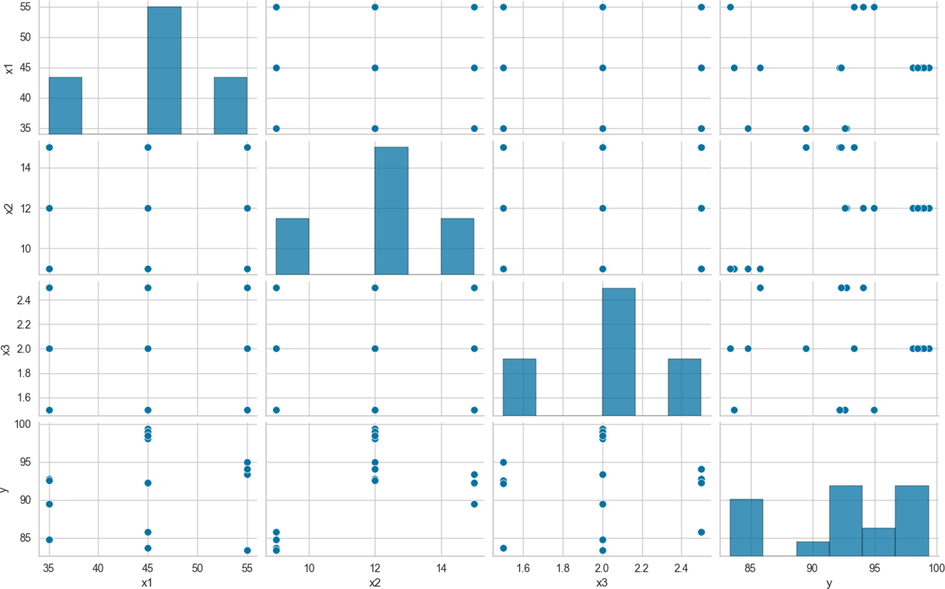
Scatter plot for Data Set of biodiesel modeling.
3 Computational methodology
3.1 CART (Classification and regression tree)
Because the decision tree (DT) estimator of the CART type is employed as a weak or basic estimator in all of the models in this study, we will first introduce the concept of this method. The decision tree method is a learning model often utilized for both regression and classification tasks. The partitioning method results in a tree-like architecture so the model is called decision tree (DT). A DT contains a root node and child (sub) nodes that include all the cases and non-cases necessary for training the model (Cheraghlou et al., 2021). Fig. 2 depicts this process graphically as a binary decision tree.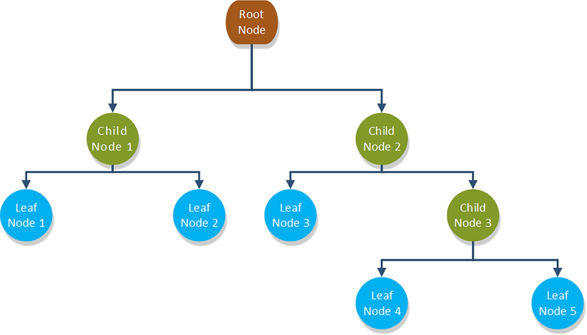
A straightforward binary decision tree structure with a three-level depth.
The splitting criterion is critical in the construction of a DT. Numerous DT algorithms employing diverse splitting criteria have been developed over the years, including the C4.5, ID3, and CART decision tree algorithms. (Quinlan, 1986, 2014). A sampling technique called CART was developed by Breiman et al. (Breiman et al., 2017; Saha et al., 2021). Impurity in a dataset can be quantified using the Gini index (GI). Using Eq. (1), we can calculate the Gini index of the node's sample set S. The GI for a node is more representative of the quality of its data if it is lower. This means that when using attribute splitting, the weighted mean of GI on each branch (sub-node) is optimised, resulting in the maximum possible value of
as defined in Eq. (2) (Liu et al., 2018).
In these equations, Ks reflects the count of outputs in the node and pk denotes the proportion of the kth category in the node. denotes the change in impurity levels between the sample set S pre-split and post-split with feature an as the split attribute (Alobaida and Huwaimel, 2023). Sample sets of left and right child nodes are denoted by SL and SR, while WL and WR represent their respective proportions. Like other DT induction techniques, CART finds the most significant variables when choosing the optimum splitting features for each root or internal node, hence defining independent variables is unnecessary (Menze et al., 2009; Shang et al., 2007). As a result, CART seems to be appropriate for learning situations in which the relationship between inputs and output is uncertain (Safavian and Landgrebe, 1991).
3.2 AdaBoost algorithm
A model based on ensemble approach is formed by combining several base (weak) models, and such a model typically outperforms a single estimator. Freund and Schapire (Freund and Schapire, 1997) proposed the AdaBoost algorithm as an ensemble model for boosting the performance of weak models by varying the distribution of sample weights. The AdaBoost main workflow as follows (Hastie et al., 2009):
-
Initialize weight values where i ∈ {1, …, N} (N stands for the quantity of input vectors).
-
construct the predictor (the tth predictor) on data points using the current weights for t = 1 to Tc. Next, the Eq. (3) is utilized to declare ε (t), the error, and calculating the weight of the predictor α (t) is done with the help of Eq. (4). Finally, Eqs. (5) and (6) are employed to modify the weights of samples (Gupta et al., 2016).
where ci stands for actual output of the ith sample, K represents the total count of possible outputs. To get a total of 1 for , the indicator function is , and Zt is the normalization factor.
Compute the final output:
After a training iteration, samples that correctly identified incorrect results are given higher weights, as shown in Eqs. (3)–(7). As a result, these examples are given greater consideration as the subsequent base learner is being trained. The model's output is a weighted average of all of its base learners.
3.3 Extremely randomized tree (ET)
Extra tree (Extremely Randomized Tree or ET) is also an ensemble model for supervised tasks (classification or regression) that is built on trees. It is a recent technique designed as a random forest extension. The ET Method builds a collection of unpruned decision tree estimators from the top down. This algorithm employs a random subset of input parameters to build each weak (base) predictor, similar to the RF technique. For each node, ET selects feature and its corresponding value at random (Ahmad et al., 2018; John et al., 2015; Gallicchio et al., 2017).
This guarantees that a sizable portion of the variance in the trained DT estimator is accounted for by the ideal cut-point. This concept is beneficial in the context of various problems with many numerical features that change over time: it frequently leads to enhanced accuracy because of the smoothing of the numerical features and a massive reduction in computational burdens associated with determining optimized cut-points in standard decision trees. As a consequence of this, in the worst-case scenario, it generates completely random trees with topologies that are unaffected by the output values of the learning sample. By selecting the proper parameter, the degree to which the randomization is applied can also be modified to correspond with the specifics of the scenario (Geurts et al., 2006).
The Extra Tree method creates a series of weak regression trees using the conventional top-down procedure. The significant dissimilarities between ET and other DT-based techniques are that it separates nodes randomly and builds the tree using the entire learning sample. The final prediction is made by combining the tree (base estimators) predictions, either by the majority of votes in classification tasks or by numerical average or weighted average in numerical regression tasks. Extra tree trains each base estimator using random subset features (John et al., 2015).
The Extremely Randomized Trees approach is predicated on the idea that explicit randomization of cut-points and features, in conjunction with ensemble averaging, efficiently eliminates contrasts and similarities. From a computational standpoint, the computational complexity of the tree growth technique (for a balanced tree) is proportional to the learning sample size in the N log N time complexity (Geurts et al., 2006; Okoro et al., 2022).
3.4 Gradient boosting regression tree (GBRT)
Valiant came up with the idea of boosting (Valiant, 1984). When we combine many weak models, we can make a strong model. This is the main concept underlying this algorithm. Friedman proposed the gradient boosting algorithm in (Friedman, 2001) with the idea that it could be employed to fit non-parametric prediction model. It is called Gradient Boosting Regression Tree (GBRT), and it uses regression tree as the base estimator. The steps of GBRT are as follows (Ikeagwuani, 2021):
-
M samples are taken from N datasets.
-
The residuals (negative gradient) for each sample are calculated.
-
Residuals are employed in training instances, and the best partition point from M-dimensional features is found by minimizing the loss function.
-
Changes occur when a new partition node generates leaf nodes with sample split.
-
If the minimum MSE is not attained, return to step 2.
The flow of each tree is as follows (Wei et al., 2019):
4 Results and discussions
In this step, after looking at the tuned hyper-parameters, the final models will be created and compared using tree metrics to evaluate and analyze the results of the suggested models:
With the help of Eq. (11), the Mean Absolute Error metric (MAE) (Botchkarev, 2018), that is the horizontal distance between two continuous variables, namely the arrays of measured and model projected Yield of FAME, is calculated.
Here, n reflects the count of input samples and yi is the observed value. Also, denotes model predicted values (Wang and Lu, 2018; Kumar et al., 2020).
The Root Mean Squared Error (RMSE) is the second indicator that was employed in the comparison (RMSE). In Eq. (12), it is stated as the standard deviation of model estimated outputs from observed values on a dataset (Kumar et al., 2020; Fajar and Sugiarto, 2012):
R2-Score, is the last metric. In regression tasks, the R2-Score (Botchkarev, 2018) is utilized to gauge how closely the model's predictions match the actual values. Equation (13) provides a relationship that can be used to compute it.
In this equation, μ stands for the average of the observed data.
For the ADA-RT model, we need to decide on nine essential hyper-parameters. Although other parameters can affect the output of our model, we have optimized these nine more essential parameters.
Table 2 lists some of the best combinations. The final optimized values for the parameters are:
-
Criterion: The function's quality is determined by this parameter. As an alternative to using mean squared error, Friedman MSE takes into account both the error and the improvement made by the split, and is therefore used for future partitions.
-
Splitter method: The mechanism used to find the split at each node. The chosen strategy is “best” for choosing the best split for identifying the appropriate random split.
-
Max depth: The maximum tree depth has been determined to be 14.
-
Minimum samples split: 6
-
Minimum samples leaf: 2
-
Maximum features: 3
-
Learning rate: 1.0
-
Number of estimators: 170
-
Loss Function: Linear
| Criterion | Splitter | Max depth | Min samples split | Min samples leaf | Max features | Learning rate | Number of trees | Loss | MAE |
|---|---|---|---|---|---|---|---|---|---|
| Absolute error | random | 5 | 2 | 2 | 2 | 1.059882353 | 119 | square | 1.216 |
| Friedman mse | best | 14 | 6 | 2 | 3 | 0.993823529 | 177 | linear | 1.187 |
| Friedman mse |
random | 12 | 3 | 2 | 2 | 0.255 | 175 | square | 1.370 |
| Friedman mse | random | 20 | 2 | 2 | 3 | 0.104058824 | 64 | exponential | 1.530 |
| Friedman mse | best | 6 | 4 | 2 | 2 | 0.767705882 | 138 | square | 1.406 |
| Squared error | best | 8 | 4 | 2 | 3 | 1.629647059 | 163 | square | 1.437 |
| Squared error | random | 18 | 2 | 2 | 3 | 2.425470588 | 82 | linear | 1.621 |
| Friedman mse | best | 3 | 5 | 2 | 2 | 1.952176471 | 114 | exponential | 1.741 |
| Friedman mse | random | 11 | 2 | 2 | 2 | 0.112823529 | 159 | exponential | 1.705 |
| Absolute error | random | 2 | 2 | 2 | 2 | 0.203588235 | 67 | linear | 1.656 |
| Friedman mse | best | 12 | 3 | 2 | 1 | 2.063882353 | 7 | linear | 1.624 |
| Friedman mse | best | 15 | 4 | 2 | 2 | 2.396 | 121 | exponential | 1.729 |
| Friedman mse | random | 13 | 6 | 2 | 3 | 1.048823529 | 57 | exponential | 2.280 |
| Absolute error | random | 5 | 2 | 3 | 2 | 1.909941176 | 72 | linear | 2.39 |
Based on all combinations tests (top results are presented in Table 3), the final hyper-parameters for the Extra tree regressor are as follows:
-
Number of estimators: 126
-
Criterion: Absolute error was chosen as the function to improve the impact of a split.
-
Max Depth: 8
-
Max Features: 3
| Number of estimators | Criterion | Max depth | Max features | MAE |
|---|---|---|---|---|
| 126 | Absolute error | 8 | 3 | 1.186 |
| 127 | Absolute error | 9 | 3 | 1.192 |
| 129 | Absolute error | 19 | 3 | 1.199 |
| 129 | Absolute error | 15 | 3 | 1.199 |
| 133 | Absolute error | 6 | 3 | 1.201 |
| 102 | Absolute error | 17 | 3 | 1.226 |
| 131 | Absolute error | 20 | 3 | 1.206 |
| 121 | Absolute error | 11 | 3 | 1.199 |
| 130 | Absolute error | 12 | 3 | 1.209 |
| 124 | Absolute error | 12 | 3 | 1.204 |
| 124 | Absolute error | 15 | 3 | 1.204 |
| 184 | Absolute error | 15 | 3 | 1.247 |
| 96 | Absolute error | 20 | 3 | 1.249 |
| 96 | Absolute error | 8 | 3 | 1.249 |
Finally, the top results for Gradient Tree Boosting may be found in Table 4. Based on these experiments, we chose the following hype-parameters:
-
Learning Rate: 1.25
-
Number of Estimators: 30
-
Tolerance for the early stopping: 2.25E−4
-
Criterion: This is the function that determines the quality of a split is set to squared error for gradient boosting.
-
Loss Function: We used the Huber Loss function to optimize the gradient tree boosting.
| Learning rate | Number of estimators | Loss | Criterion | Tol | MAE |
|---|---|---|---|---|---|
| 1.208118 | 197 | huber | mse | 0.000243 | 0.221 |
| 1.261 | 30 | huber | Squared error | 0.000225 | 0.197 |
| 1.255647 | 147 | huber | Friedman mse | 1.49E-05 | 0.215 |
| 1.264235 | 9 | huber | Friedman mse | 7.04E-05 | 0.230 |
| 1.264647 | 12 | huber | Friedman mse | 9.05E-05 | 0.229 |
| 1.255471 | 90 | huber | Squared error | 0.000102 | 0.243 |
| 1.258235 | 200 | huber | Squared error | 0.000137 | 0.236 |
| 1.199235 | 192 | huber | Friedman mse | 0.00026 | 0.294 |
| 1.269765 | 6 | huber | Friedman mse | 2.80E-05 | 0.277 |
| 1.160647 | 115 | huber | Mse | 9.26E-05 | 0.304 |
| 1.195706 | 43 | huber | Squared error | 8.02E-05 | 0.289 |
| 1.165059 | 188 | huber | Friedman mse | 0.000221 | 0.351 |
| 1.233176 | 41 | huber | Friedman mse | 6.65E-05 | 0.343 |
| 1.156412 | 127 | huber | Friedman mse | 4.83E-05 | 0.374 |
| 1.251706 | 67 | huber | Mse | 2.03E-05 | 0.351 |
| 1.205118 | 90 | huber | Squared error | 9.29E-05 | 0.329 |
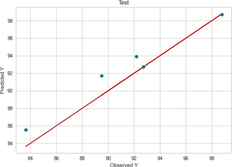
The observed and predicted FAME yield production according to the ADA + RT model are presented in Figs. 3 and 4 for train and test values, respectively. As can be seen a good accuracy was obtained from this model in the training phase. However, according to Fig. 4, in ADA + RT model testing phase the distance between the actual and predicted values was increased in some values.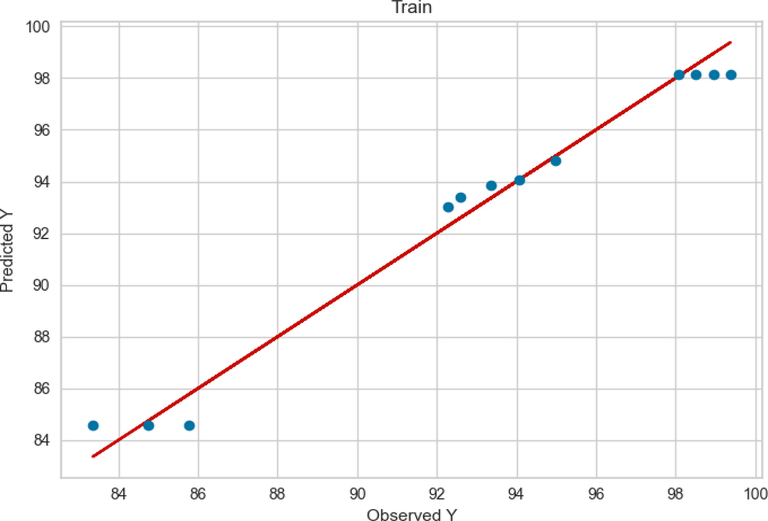
Train results of ADA + RT.
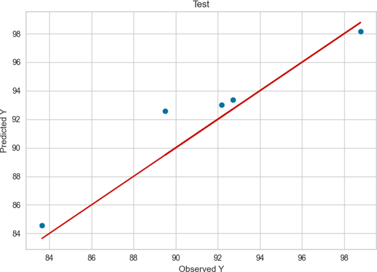
Test results of ADA + RT.
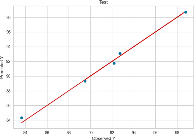
The result of Extra Tree model for the train and test data are presented in Figs. 5 and 6, respectively. By comparing Fig. 3 and Fig. 5 it can be said that both models had a large extent in the training phase. Same as ADA + RT model, the Extra Tree model had better performance and more accuracy in learning step however, the ADA + RT Extra Tree model (Fig. 6) performance in test phase was better than ADA + RT model in the same phase (Fig. 4).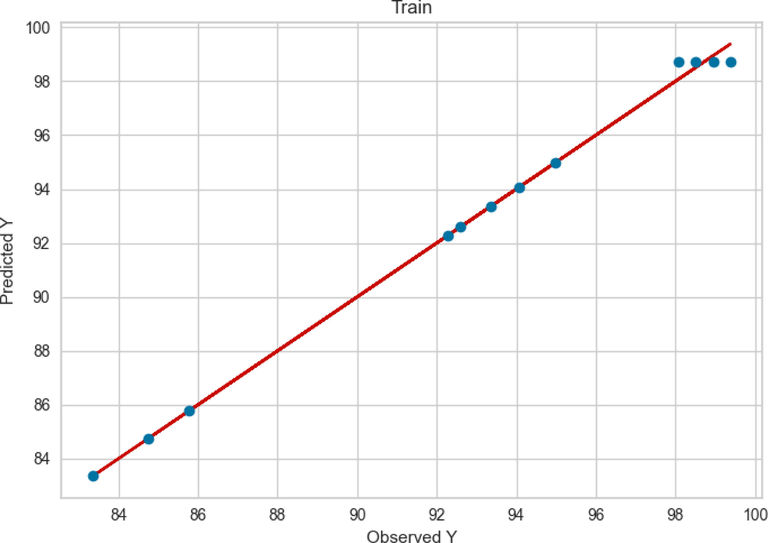
Train results of Extra Tree.
Test results of Extra Tree.
Similarly, the observed and predicted FAME yield production by GBRT model in the train and test phase are presented in Figs. 7 and 8, respectively. Compared to ADA + RT and Extra Tree models, the GBRT model performance was better in both train and test phase. As can be seen in Figs. 7 and 8, the observed and the predicted values in the GBRT model were more accurate. model in this phase can be observed compared to the previous two models (Figs. 3 and 5).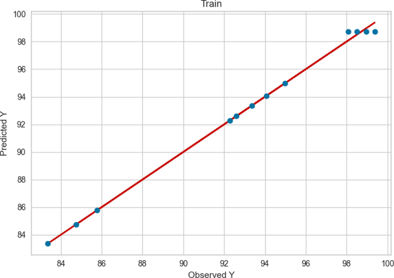
Train results of GBRT.
Test results of GBRT.
For evaluation of models MAE, R-square, and RMSE were calculated for each model. These coefficients represent how well the model fits compared to the real values. The obtained results are illustrated in Table 5. As is obvious in this Table, the R2 values of 0.979, 0.997, and 0.997 were obtained for ADA + RT, Extra Tree, and GBRT models, respectively. The higher R2 value specifies a better fit in model results, therefore, it can be concluded that the Extra Tree, and GBRT models can fit the data better than ADA + RT model. The RMSE error rates for the ADA + RT, Extra Tree, and GBRT models were obtained as 1.549, 1.524, and 0.396, respectively. Also, lower MAE value was attained for GBRT model (0.333) while ADA + RT and Extra Tree models had higher MAE values (1.224 and 1.186, respectively). According to the obtained results it can be said that the GBRT model had more accurate prediction and more properly model the FAME production yield data compared to the ADA + RT and Extra Tree models. As a result, the following section will delve deeper into this particular model. This can also be confirmed by Fig. 9, which shows the residuals of this model.
Models
MAE
R2
RMSE
AdaBoosted Regression Tree
1.224
0.979
1.549
Extra Trees
1.186
0.997
1.524
Gradient boosting regression tree
0.333
0.997
0.396
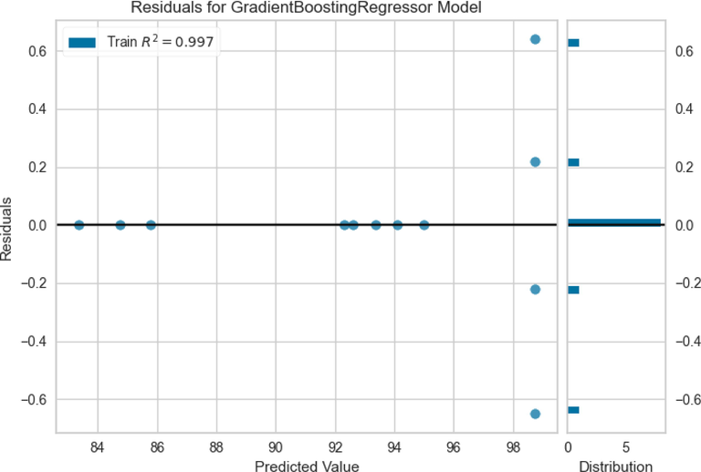
Residuals of prediction using GBRT model.
Further information in the form of 3D diagrams about the impact of operational factors on the FAME production yield is provided in Figs. 10–12. These two-way relationships between operating factors and FAME yield are visualized here with the help of GBRT model output. Fig. 10 represents the dual effect of reaction time and methanol to oil ratio on the biodiesel production yield while the third factor (catalyst amount) was fixed at the value of 2 wt%. Increasing the molar ratio increases the content of methanol in the reaction media and leads to higher production of biodiesel (Abdelbasset et al., 2022). However, as can be seen when the amount of methanol increased too much in the reaction media the production yield decreased. The higher amount of methanol lead to fact consumption of oil content in the system which decrease the FAME production (Yang et al., 2009). Therefore, the optimum amount of methanol to oil molar ration should be obtained.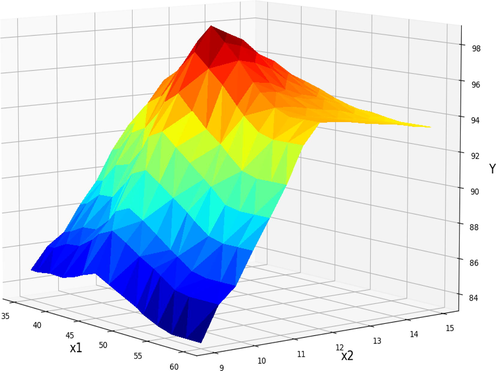
Projection of X1 and X2 in final GBRT model. X3 = 2 kept Constant. Optimum value is y = 98.72 for x1 = 45, x2 = 12.
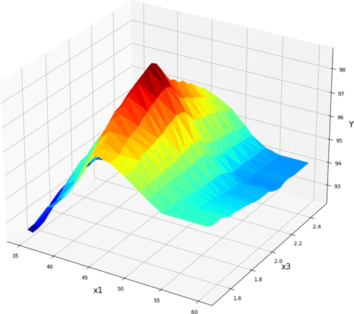
Projection of X1 and X3 in final GBRT model. X2 = 12 kept Constant. Optimum value is y = 98.72 for x1 = 45, x3 = 2.
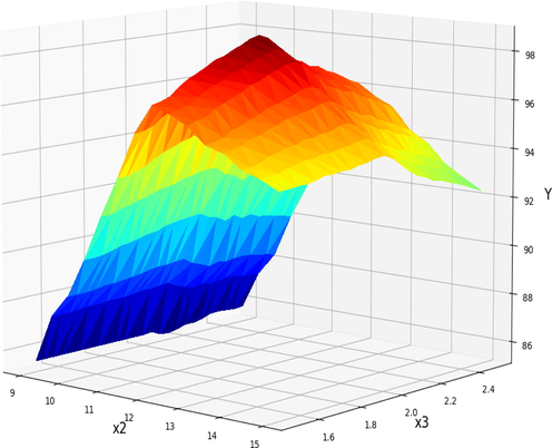
Projection of X2 and X3 in final GBRT model. X1 = 45 kept Constant. Optimum value is y = 98.73 for x2 = 12, x3 = 1.95.
Keeping the molar ratio of methanol to oil at 12 and varying the reaction time and amount of catalyst, Fig. 11 displays the combined effect on FAME production yield. As can be seen, the production of FAME went up as the amount of catalyst went up. However, biodiesel production is hampered after a certain threshold of catalyst higher increment. There can be a transesterification reaction if enough basic sites are provided when the catalyst amount is increased to a certain value. However, the biodiesel production yield is reduced when the catalyst amount is increased to a point where there is too much resistance in the reaction flow (Zhang et al., 2020; Li et al., 2013). Transesterification is a reversible reaction and at the equilibrium point the maximum yield of biodiesel could be obtained. In long period of reaction times the transesterification can be performed in the reverse direction and reduce the production yield.
Fig. 12 describes the dual influence of methanol to oil molar ratio and catalyst amount on the FAME generation rate while the reaction time was kept constant at 45 h. As can be seen at lower amount of catalyst and methanol to oil molar ratio the FAME production yields were low. This can be because of fast consumption of methanol and catalyst during the reaction. By increasing the amount of catalyst and the methanol-to-oil molar ratio, FAME production yields can be increased; however, biodiesel production reaches a maximum and then declines. This can be explained by the possibility of side reactions that consume methanol and catalyst (Abdelbasset et al., 2022; Chopade et al., 2012; Vicente et al., 2007). In order to obtain the maximum quantity of biodiesel production, it is evident that the ideal amount of catalyst and methanol to oil molar ratio should be calculated.
The impact of each variable on the yield of FAME was shown in Figs. 13–15. By keeping the other factors constant, the one unique impact of each variable on biodiesel production can be obtained as 2D diagrams. These findings are consistent with those found in Figs. 10–12.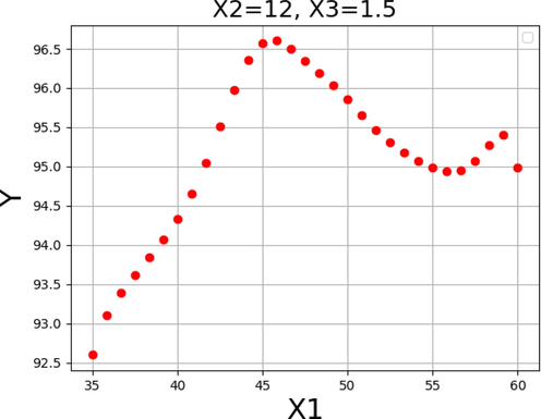
Response tendency for x1.
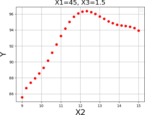
Response tendency for x2.
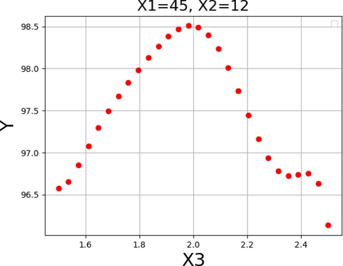
Response tendency for x3.
In general, these results suggest an increase in reaction to values that are near to those shown in Table 6 for each of the input variables. Thus, the pattern in these three data supports the validity of the optimizations in Table 6 as a whole. As can be seen, the maximum biodiesel production yield of 99.729% is achievable under the following optimized conditions: reaction time of 45 h, methanol to oil molar ratio of 12.0, and catalyst amount of 2.0 wt%.
X1: Reaction time (h)
X2: Methanol: oil
X3: Catalyst amount (wt.%)
Y: Yield of FAME (%)
45
12.0
2.0
98.729
5 Conclusion
Biodiesel production from oil was optimized in this work using a number of machine learning models. The models for the optimization included AdaBoost (DT base), Extra Trees, and Gradient boosting regression tree (GBRT). The R2, RMSE, and MAE are metrics used to evaluate the developed regression models. According to the R-square criterion, all three models selected for this study had R2 value greater than 0.9, which demonstrate the accuracy of assembled models. However, in terms of MAE and RMSE the GBRT had the lowest values (0.333 and 0.396, respectively) compared to ADA + RT (1.224 and 1.549, respectively) and Extra Trees (1.186 and 1.524, respectively) models. Although the three developed models were accurate and properly predict biodiesel production, the GBRT model was determined as the most appropriate model for further investigations. The results indicated that a maximum biodiesel production yield of 99.729% may be achieved under the ideal conditions of 45 h of reaction time, a methanol to oil molar ratio of 12.0, and a catalyst quantity of 2.0 wt%. The promising results of this study confirmed that ML techniques can provide new opportunities to enhance biodiesel production efficiency and reduce the overall time and cost of processes.
Declaration of Competing Interest
The authors declare that they have no known competing financial interests or personal relationships that could have appeared to influence the work reported in this paper.
References
- Optimization of heterogeneous Catalyst-assisted fatty acid methyl esters biodiesel production from Soybean oil with different Machine learning methods. Arab. J. Chem.. 2022;15(7):103915
- [Google Scholar]
- Machine learning technology in biodiesel research: A review. Prog. Energy Combust. Sci.. 2021;85:100904
- [Google Scholar]
- Trees vs Neurons: Comparison between random forest and ANN for high-resolution prediction of building energy consumption. Energy Build.. 2017;147:77-89.
- [Google Scholar]
- Tree-based ensemble methods for predicting PV power generation and their comparison with support vector regression. Energy. 2018;164:465-474.
- [Google Scholar]
- Raw material for biodiesel production. Valorization of used edible oil. J. Renewable Energies. 2014;17(2):335-343.
- [Google Scholar]
- Analysis of enhancing drug bioavailability via nanomedicine production approach using green chemistry route: Systematic assessment of drug candidacy. J. Mol. Liq.. 2023;370:120980
- [Google Scholar]
- Application of machine learning in anaerobic digestion: Perspectives and challenges. Bioresour. Technol.. 2022;345:126433
- [Google Scholar]
- Modeling of cetane number of biodiesel from fatty acid methyl ester (FAME) information using GA-, PSO-, and HGAPSO-LSSVM models. Renew. Energy. 2020;150:924-934.
- [Google Scholar]
- Botchkarev, A., 2018. Evaluating performance of regression machine learning models using multiple error metrics in azure machine learning studio. Available at SSRN 3177507.
- Classification and regression trees. Routledge; 2017.
- A machine-learning modified CART algorithm informs Merkel cell carcinoma prognosis. Australas. J. Dermatol. 2021
- [Google Scholar]
- Solid heterogeneous catalysts for production of biodiesel from trans-esterification of triglycerides with methanol: a review. Acta Chim. Pharm. Indica. 2012;2(1):8-14.
- [Google Scholar]
- Machine learning for credit scoring: Improving logistic regression with non-linear decision-tree effects. Eur. J. Oper. Res.. 2022;297(3):1178-1192.
- [Google Scholar]
- Predicting fuel properties of partially hydrogenated jatropha methyl esters used for biodiesel formulation to meet the fuel specification of automobile and engine manufacturers. Agric. Natural Resour.. 2012;46(4):629-637.
- [Google Scholar]
- Ferreira, A.J., Figueiredo, M.A.T., 2012. Boosting Algorithms: A Review of Methods, Theory, and Applications, in Ensemble Machine Learning: Methods and Applications, C. Zhang and Y. Ma, Editors. Springer US, Boston, MA. pp. 35–85.
- Freund, Y., Schapire, R.E., 1996. Experiments with a new boosting algorithm. In: icml. Citeseer.
- A decision-theoretic generalization of on-line learning and an application to boosting. J. Comput. Syst. Sci.. 1997;55(1):119-139.
- [Google Scholar]
- Greedy function approximation: a gradient boosting machine. Ann. Stat. 2001:1189-1232.
- [Google Scholar]
- Gallicchio, C., et al., 2017. Randomized Machine Learning Approaches: Recent Developments and Challenges. In: ESANN.
- A new transfer learning framework with application to model-agnostic multi-task learning. Knowl. Inf. Syst.. 2016;49(3):933-973.
- [Google Scholar]
- Estimation of modified expansive soil CBR with multivariate adaptive regression splines, random forest and gradient boosting machine. Innov. Infrastruct. Solut.. 2021;6(4):1-16.
- [Google Scholar]
- Impacts of derivatization on physiochemical fuel quality parameters of fatty acid methyl esters (FAME)-a comprehensive review. Int. J. Chem. Biochem. Sci. 2019;15:42-49.
- [Google Scholar]
- Modern multivariate statistical techniques. Regress. Classif. Manifold Learn.. 2008;10:978.
- [Google Scholar]
- Current scenario of catalysts for biodiesel production: A critical review. Rev. Chem. Eng.. 2018;34(2):267-297.
- [Google Scholar]
- Real-time lane estimation using deep features and extra trees regression. In: Image and Video Technology. Springer; 2015.
- [Google Scholar]
- Production and optimization from Karanja oil by adaptive neuro-fuzzy inference system and response surface methodology with modified domestic microwave. Fuel. 2021;296:120684
- [Google Scholar]
- Optimization at low temperature transesterification biodiesel production from soybean oil methanolysis via response surface methodology. Energy Sources Part A. 2022;44(1):2284-2293.
- [Google Scholar]
- A machine learning-based model to estimate PM2.5 concentration levels in Delhi's atmosphere. Heliyon. 2020;6(11)
- [Google Scholar]
- Experimental Study on Biodiesel Production Parameter Optimization of Jatropha-Algae Oil Mixtures and Performance and Emission Analysis of a Diesel Engine Coupled with a Generator Fueled with Diesel/Biodiesel Blends. ACS Omega. 2020;5(28):17033-17041.
- [Google Scholar]
- Application of adaptive neuro-fuzzy inference system and response surface methodology in biodiesel synthesis from jatropha–algae oil and its performance and emission analysis on diesel engine coupled with generator. Energy. 2021;226:120428
- [Google Scholar]
- A stirring packed-bed reactor to enhance the esterification–transesterification in biodiesel production by lowering mass-transfer resistance. Chem. Eng. J.. 2013;234:9-15.
- [Google Scholar]
- Accuracy analyses and model comparison of machine learning adopted in building energy consumption prediction. Energy Explor. Exploit.. 2019;37(4):1426-1451.
- [Google Scholar]
- A novel method for identifying influential nodes in complex networks based on multiple attributes. Int. J. Mod. Phys. B. 2018;32(28):1850307.
- [Google Scholar]
- A comparison of random forest and its Gini importance with standard chemometric methods for the feature selection and classification of spectral data. BMC Bioinf.. 2009;10(1):1-16.
- [Google Scholar]
- Application of artificial intelligence in predicting the dynamics of bottom hole pressure for under-balanced drilling: Extra tree compared with feed forward neural network model. Petroleum. 2022;8(2):227-236.
- [Google Scholar]
- A decision tree algorithm pertaining to the student performance analysis and prediction. Int. J. Comput. Appl.. 2013;61(13)
- [Google Scholar]
- A Review of Classification Problems and Algorithms in Renewable Energy Applications. Energies. 2016;9
- [CrossRef] [Google Scholar]
- Experimental study of the factors affecting the oxidation stability of biodiesel FAME fuels. Fuel Process. Technol.. 2014;125:223-235.
- [Google Scholar]
- Quinlan, J.R., 2014. C4. 5: programs for machine learning. Elsevier.
- Ensemble approach based on bagging, boosting and stacking for short-term prediction in agribusiness time series. Appl. Soft Comput.. 2020;86:105837
- [Google Scholar]
- A survey of decision tree classifier methodology. IEEE Trans. Syst. Man Cybern.. 1991;21(3):660-674.
- [Google Scholar]
- Comparison between Deep Learning and Tree-Based Machine Learning Approaches for Landslide Susceptibility Mapping. Water. 2021;13(19):2664.
- [Google Scholar]
- A novel feature selection algorithm for text categorization. Expert Syst. Appl.. 2007;33(1):1-5.
- [Google Scholar]
- Optimisation of integrated biodiesel production. Part I. A study of the biodiesel purity and yield. Bioresour. Technol.. 2007;98(9):1724-1733.
- [Google Scholar]
- Analysis of the Mean Absolute Error (MAE) and the Root Mean Square Error (RMSE) in Assessing Rounding Model. IOP Conf. Ser.: Mater. Sci. Eng.. 2018;324(1):012049
- [Google Scholar]
- An improved gradient boosting regression tree estimation model for soil heavy metal (arsenic) pollution monitoring using hyperspectral remote sensing. Appl. Sci.. 2019;9(9):1943.
- [Google Scholar]
- Decision tree regression for soft classification of remote sensing data. Remote Sens. Environ.. 2005;97(3):322-336.
- [Google Scholar]
- Catalytic properties of a lipase from Photobacterium lipolyticum for biodiesel production containing a high methanol concentration. J. Biosci. Bioeng.. 2009;107(6):599-604.
- [Google Scholar]
- Biodiesel production from palm oil and methanol via zeolite derived catalyst as a phase boundary catalyst: An optimization study by using response surface methodology. Fuel. 2020;272:117680
- [Google Scholar]
- Environmental impacts the of production and use of biodiesel. Environ. Sci. Pollut. Res.. 2018;25(1):191-199.
- [Google Scholar]


