

Translate this page into:
Presenting the best correlation relationship for predicting the dynamic viscosity of CuO nanoparticles in ethylene glycol -water base fluid using response surface methodology
⁎Corresponding author. Toghraee@iaukhsh.ac.ir (Davood Toghraie)
-
Received: ,
Accepted: ,
This article was originally published by Elsevier and was migrated to Scientific Scholar after the change of Publisher.
Abstract
Using response surface methodology (RSM) statistical method. 2FI, Quadratic, Cubic and Quartic models were investigated in this study. The Quartic model was chosen as the superior model and was used to optimize the NF viscosity. The optimization was done in cold environmental conditions.
Abstract
The types of correlation relationships by different models for predicting of the dynamic viscosity of CuO nanoparticles (NPs) in the ethylene glycol (EG) (80 %)-Water (20 %) base fluid (BF) by using response surface methodology (RSM) statistical method under temperature conditions of T = 15 to 50 °C, solid volume fractions of SVF = 0.05 to 1 % and shear rate SR = 26.6 to 933.1 s−1 were investigated. Models of Quadratic, Cubic, 2FI and Quartic were investigated. These different models were analyzed based on the measurement criteria such as Correlation deviation, coefficient of determination, standard deviation, reliability and P-values; there are important parameters that were used to compare the models. Among these four models, the Quartic model has been chosen as superior model and used to optimize nanofluid (NF) viscosity. The optimization was done in cold environmental conditions and SVF, T, SR variables and viscosity were selected as minimum values and applied to the system. In the conditions of T = 25.303 °C, SVF = 0.05 % and SR = 26.660 sec-1, most optimal NF viscosity value was 8.565 mPa.sec.
Keywords
Rheological behavior
Dynamic viscosity CuO
Ethylene glycol-Water
RSM
Nanoparticles

- R -Squared (R2)
-
Coefficient of Determination
- Adjusted R- Squared
-
Adjusted Coefficient of Determination
- Predicted R – Squared
-
Predicted Coefficient of Determination
- C.V
-
Coefficient of variation
- C.D
-
Correlation deviation
- Std. Dev
-
Standard deviation
- P-value
-
Probability value
- RSM
-
Response surface methodology
- ANN
-
Artificial neural network
- Eq
-
Equation
- HN
-
Hybrid nanofluid
- NPs
-
Nanoparticles
- MWCNTs
-
Multi-walled carbon nanotubes
- CNTs
-
carbon nanotubes
- SVF
-
solid volume fraction
- SR
-
Shear rate
- EG
-
Ethylene glycol
- (mPa.sec)
-
Viscosity
- T(°C)
-
Temperature
-
solid volume fractions
- NFs
-
nanofluids
Abbreviations
1 Introduction
Today, modelling of properties of mixtures is seen in medical sciences, mathematics, biology, chemistry, physics, etc. (Alizadeh et al., 2023; Dai et al., 2023; Ruhani et al., 2022). Nanofluid (NF) was first introduced by Choi in 1995 (Dai et al., 2023). NFs are expanded liquids that are obtained by combining nanoparticles (NPs) with 1 to 100 nm size in a base fluid. Adding NPs to base fluids (BFs) improves thermophysical properties. The use of NFs has a wide role in various scientific and industrial fields and improves heat transfer properties. Adding NPs to BFs increases thermal conductivity (TC) and viscosity of NPs compared to BFs. Many studies were done by researchers in this field (Apmann et al., 2021; de Oliveira et al., 2019; Omrani et al., 2019; Urmi et al., 2022; Younes et al., 2022; Choi and Eastman, 1995). NF is used in heat exchangers, cooling, chillers and many industries (Li et al., 2020; Krishnakumar et al., 2019; Elfaghi and Hisyammudden, 2021; Pordanjani et al., 2019; Arora and Gupta, 2020). The combination of water and ethylene glycol (EG) has an acceptable performance at different temperatures and conditions and increases and improves heat transfer (HT) rate. This compound is used as a BF in many energy systems because of the high heat capacity of water and protection against EG corrosion. Many studies were done in the field of adding NPs to BFs of water, EG or a mixture of them (Kazem et al., 2021; Khan et al., 2019; Neves et al., 2022; Ramadhan et al., 2021; Vallejo et al., 2019). Many studies were done by researchers on NFs effect on dynamic viscosity. In Table 1, some studies on dynamic viscosity NF effect are presented.
Ref.
Author
NF
BF
method
Results
(Fan et al., 2022)
Asadi et al.
CuO-TiO2
water
Experimental
maximum dynamic viscosity at SVF = 1 % and T = 25 °C, and also prepared NF had a Newtonian behavior.
(Ramadhan et al., 2021)
Hemmat Esfe et al.CuO
EG
Experimental, ANN
Sensitivity analysis shows that SVF has a greater effect on viscosity.
(Asadi et al., 2020)
Ghasemi et al.
CuO
liquid paraffin
Experimental
NF viscosity is more sensitive to SVF compared to temperature
(Esfe et al., 2018)
Ahmadi et al.
CuO
water
M5-tree, MPR, ANN-MLP, GMDH, and MARS
The value of R2 and AAPR with ANN-MLP model are 0.9997 and 1.312 %, respectively.
(Ghasemi and Karimipour, 2018)
Kole et al
CuO
gear oil
Experimental
The viscosity of NFs increases with decreasing temperature and increasing SVF.
(Ahmadi et al., 2020)
Karimipour et al
CuO
liquid paraffin
ANN
Dynamic viscosity NF ratio to BF viscosity decreases significantly by increasing T and increases by increasing of SVF.
Hemmat et al. (Kole and Dey, 2011) by adding MWCNT, SiO2 NPs to 5 W50 engine oil as a BF, investigated dynamic viscosity NF experimentally in T conditions between 5 and 55 °C, SR between 50 and 800 rpm and SVF between 0 and 1 %. For example, coefficient of determination was R2 = 0.9914, which indicates a favorable value. Hemmat Esfe et al. (Karimipour et al., 2018) experimentally investigated dynamic viscosity of MWCNT-MgO / SAE40 engine oil NF. Obtained results from examining the graphs of NF viscosity in SR terms show that NF has a non-Newtonian behavior. Increasing temperature increases this non-Newtonian behavior. In the study conducted by Ghasemi et al. (Asadi et al., 2020) show that NF viscosity is more sensitive to SVF compared to temperature. Also, increasing T decreases NF dynamic viscosity. When SVF of CuO is higher than 1.5 %, viscosity increases. While SVF less than 1.5 %, the viscosity did not change much. Finally, using regression analysis, they obtained a unique statistical correlation that included temperature and SVF. Hemmat Esfe et al. (Esfe and Arani, 2018) investigated NF dynamic viscosity by using CuO and MWCNT NPs in 10 W40 motor oil as BF. Their study was done in the conditions of SVF = 0.05 to 1 % and T = 5–––55 °C. Increase in SVF increases NF viscosity compared to pure lubricant; so that maximum increase of 43.52 % in NF dynamic viscosity was achieved at SVF = 1 %. They used a statistical correlation 0.9846 with a 2th order accuracy to estimate NF viscosity. Khetib et al. (Esfe and Esfandeh, 2018) investigated the viscosity of CuO-liquid paraffin NF using RSM and ANN methods. In their study, a third-order model was selected and evaluated by ANOVA in the RSM. Comparing the results of these two methods shows that ANN method is better than RSM to predict NF viscosity. RSM is an experimental methods. This method is one of the statistical and mathematical methods to build a model. In this study, RSM is used to predict NF viscosity using CuO NPs in EG-Water base fluid. Fig. 1 shows RSM method schematic.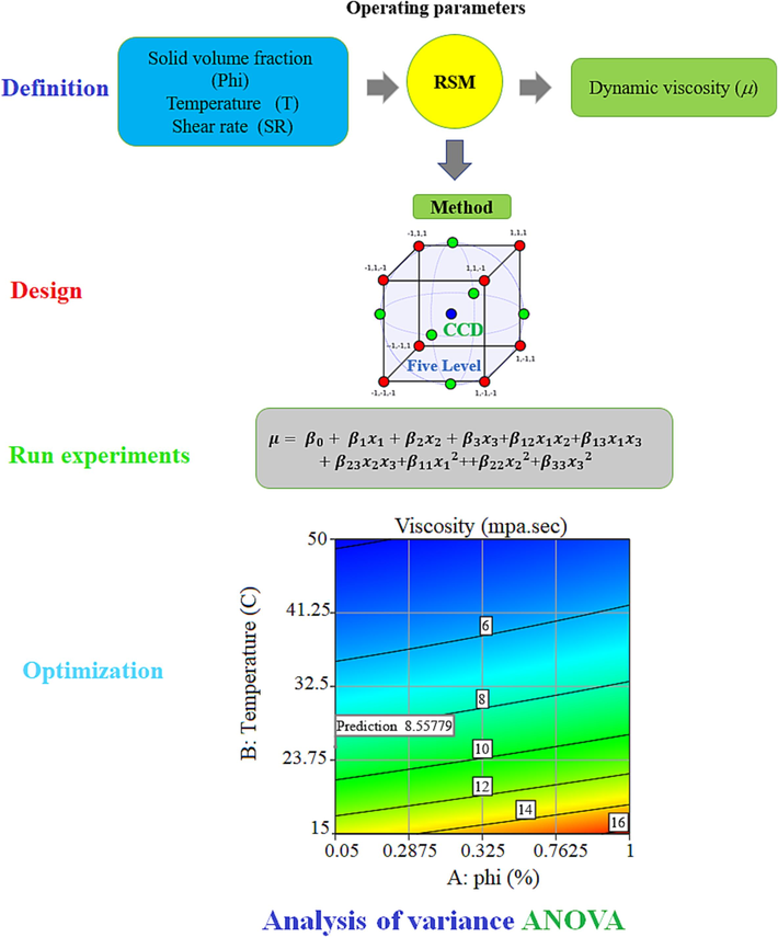
Schematic of RSM in design of experiment method.
Bhat et al. (Esfe and Sarlak, 2017) investigated NF viscosity using CuO NPs with sizes of 15, 45 and 75 nm. In this study, NF viscosity has been measured in SVF = 1–––4 % and T = 293–––353 K. Increasing T from 293 to 353 K leds to decrease of about 80 % in NF dynamic viscosity. 0.5 % increase in viscosity with an increase in SVF. Hemmat Esfe et al. (Khetib et al., 2021) investigated NF dynamic viscosity by adding MWCNT, ZrO2 NPs to 5 W50 engine oil at T = 5–––55 °C and SVF = 0.05 to 1 % to improve performance of NF. There is 20 % reduction in dynamic viscosity at SVF = 0.05 %. Also, in SVFs below 0.75 %, the viscosity decreases compared to BF. Hemmat Esfe et al. (Ramadhan et al., 2021) investigated CuO-EG dynamic viscosity NF at T = 27.5–––50 °C and SVFs = 0–––1 % using experimental and ANN methods. NF viscosity increases with increasing of SVF and decreasing of T. The results also show that the effect of temperature is significant in low SVFs. In this model selected by ANN, it was estimated with an R2 = 0.999 and an average relative error = 0.0175, which had an allowed match with tests. Also, sensitivity analysis shows that the SVF has a greater effect on the dynamic viscosity of NF than temperature. In this study, 200 experimental data have been used to optimize the dynamic viscosity of CuO nanoparticles in EG (80 %)-Water (20 %) base fluid using RSM. The aim is to obtain a correlation relationship to predict NF dynamic viscosity. To obtain this correlation coefficient, different Quadratic, Cubic, 2FI and Quartic models are used, and best model is selected by comparing some accuracy indicators and quality determination, and NF optimization is done based on selected model. After obtaining correlation relationship, NF viscosity can be obtained at different temperatures and SVFs, which saves time and money.
2 RSM statistical method
One of the mathematical and statistical methods for experiment design is the RSM. In this method, different mathematical models are used to check the influence of independent input variables and optimizing of response. To use this method, experiments with different levels of Moore's variables must be performed and data related to them must be collected. Then, using mathematical models related to the RSM, the optimal response is estimated for different values of the variables. Among the advantages of this method, we can mention the possibility of analyzing the interactions of input variables and their influence on response variable. Also, by using this method, the optimal answer can be reached with the least effort and the shortest time. Therefore, it saves time and money. In the present study, using the RSM, the following items are examined:
-
Check different models
-
Examining some indicators and model validation charts
-
Compare different models and choose the best model
-
NF viscosity optimization using superior model
2.1 Different models
2.1.1 2FI model
The correlation created by the 2FI model to predict NF viscosity values is shown in Ea. 1. This equation includes independent input parameters and interaction between these input variables. Table 2. It shows the independent input parameters and the interaction between these parameters using ANOVA analysis. In Table 3, some parameters and validation indices for the 2FI model are presented.
Source
Sum of Squares
df
Mean Square
F-value
P-value
Model
2060.10
5
412.02
944.12
< 0.0001
significant
A-
31.14
1
31.14
71.36
< 0.0001
B-T
472.90
1
472.90
1083.62
< 0.0001
C-
27.22
1
27.22
62.37
< 0.0001
AB
7.57
1
7.57
17.35
< 0.0001
BC
32.37
1
32.37
74.18
< 0.0001
Residual
84.66
194
0.4364
Cor Total
2144.76
199
Std. Dev.
0.6606
R-Squared
0.9605
Mean
7.94
Adjusted R2
0.9595
C.V. %
8.32
Predicted R2
0.9572
p-value
4.80109569518e-134
Adeq Precision
113.3196
2.1.2 Quadratic model
In Eq. (2) and Table 4, independent input variables and interaction are presented by ANOVA analysis. In Table 5, some parameters and validation indices for the Quadratic model are presented.
Source
Sum of Squares
df
Mean Square
F-value
P-value
Model
2136.72
5
427.34
10312.03
< 0.0001
significant
A-
11.72
1
11.72
282.90
< 0.0001
B-T
262.93
1
262.93
6344.64
< 0.0001
AB
14.48
1
14.48
349.33
< 0.0001
A2
0.1975
1
0.1975
4.77
0.0302
B2
109.75
1
109.75
2648.30
< 0.0001
Residual
8.04
194
0.0414
Cor Total
2144.76
199
Std. Dev.
0.2036
R-Squared
0.9963
Mean
7.94
Adjusted R2
0.9962
C.V. %
2.56
Predicted R2
0.9959
P-value
3.36147981671e-233
Adeq Precision
329.0804
2.1.3 Cubic model
The correlation created by the input independent variables and the interaction between these variables to predict NF viscosity values for the Cubic model is presented in Eq. (3). Analysis of ANOVA for Cubic model is reported in Table 6. In Table 7, some important validation parameters for the Cubic model are presented.
Source
Sum of Squares
df
Mean Square
F-value
P-value
Model
2141.98
10
214.20
14557.18
< 0.0001
significant
A-
6.75
1
6.75
458.79
< 0.0001
B-T
23.97
1
23.97
1629.10
< 0.0001
C- SR
0.2387
1
0.2387
16.22
< 0.0001
AB
2.14
1
2.14
145.36
< 0.0001
BC
0.1740
1
0.1740
11.82
0.0007
A2
0.1829
1
0.1829
12.43
0.0005
B2
6.53
1
6.53
443.85
< 0.0001
AB2
0.8435
1
0.8435
57.32
< 0.0001
B2C
0.1300
1
0.1300
8.84
0.0033
B3
2.47
1
2.47
167.98
< 0.0001
Residual
2.78
189
0.0147
Cor Total
2144.76
199
Std. Dev.
0.1213
R-Squared
0.9987
Mean
7.94
Adjusted R2
0.9986
C.V. %
1.53
Predicted R2
0.9985
P-value
5.32248028411e-267
Adeq Precision
433.5400
2.1.4 Quartic model
The correlation created by the input independent variables and the interaction between these variables for Quartic model is presented in Eq. (4). In Table 8, input variables and interaction between them that affect the viscosity of NF (response variable) are provided by ANOVA analysis for the Quartic model. In Table 9, some important validation parameters for the Quartic model are presented.
Source
Sum of Squares
df
Mean Square
F-value
P-value
Model
2142.48
13
164.81
13440.48
< 0.0001
significant
A-
1.20
1
1.20
98.07
< 0.0001
B-T
2.31
1
2.31
188.19
< 0.0001
C-
0.2670
1
0.2670
21.78
< 0.0001
AB
0.2261
1
0.2261
18.44
< 0.0001
BC
0.1912
1
0.1912
15.60
0.0001
A2
0.1784
1
0.1784
14.55
0.0002
B2
0.6009
1
0.6009
49.00
< 0.0001
AB2
0.0721
1
0.0721
5.88
0.0163
B2C
0.1454
1
0.1454
11.86
0.0007
B3
0.2256
1
0.2256
18.39
< 0.0001
AB3
0.0336
1
0.0336
2.74
0.0996
B3C
0.1166
1
0.1166
9.51
0.0024
B4
0.1053
1
0.1053
8.58
0.0038
Residual
2.28
186
0.0123
Cor Total
2144.76
199
Std. Dev.
0.1107
R-Squared
0.9989
Mean
7.94
Adjusted R2
0.9989
C.V. %
1.39
Predicted R2
0.9987
P-value
8.49355472751e-269
Adeq Precision
424.6076
2.2 Important parameters for determining model quality
The evaluation of important validation parameters such as correlation deviation, standard deviation, coefficient of determination, reliability and P-values for different models are examined in this section.
2.2.1 Correlation deviation parameter
Correlation deviation (C.D %) is one of the measurement criteria to show the degree of overlap between obtained software data and tests. C.D% is the points on the correlation line (measurement criterion line) in a two-variable data (data obtained from software and experimental work). This deviation indicates the deviation of the data from the correlation line. A positive correlation deviation means that the points are above the correlation line and a negative correlation deviation means that the points are below the correlation line. Therefore, the highest correlation deviation of C.D% means the highest overturning or deviation of the points from the correlation line. Eq. (5) is used to calculate correlation deviation. In Fig. 2, C.D% and deviation range are presented for four different models and Quartic model is more accurate in Fig. 2and the range of data deviation is smaller in this model.
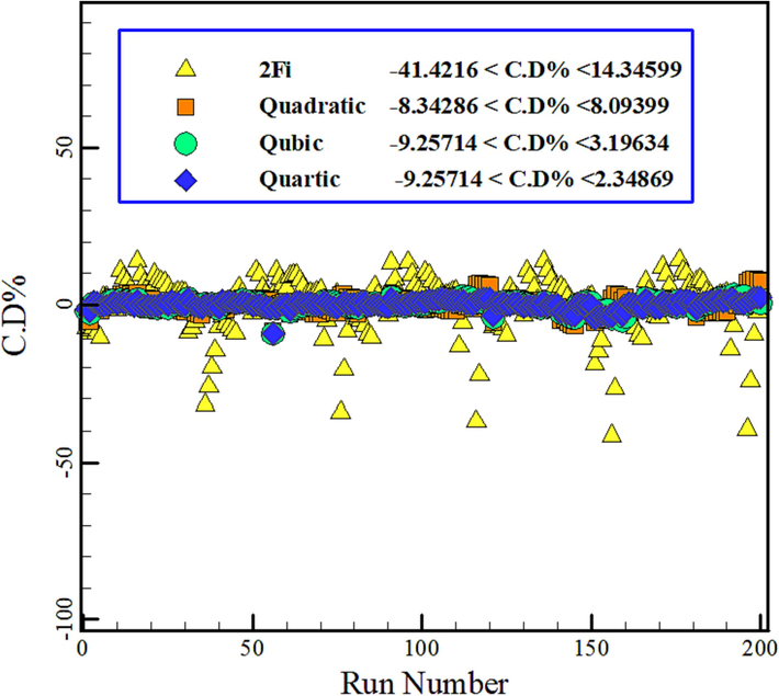
Correlation deviation for 4 different models.
2.2.2 Standard deviation parameter
One of the applied criteria in statistics and probabilities is standard deviation. The smaller the correlation deviation is, it indicates that the dispersion of the data is closer to the mean value and has higher accuracy. In Fig. 3, standard deviation is plotted for four models. As it is clear from Fig. 3, standard deviation value is smaller for Quartic model, which shows the high accuracy of this model.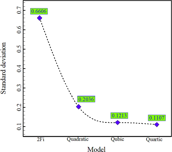
Standard deviation for 4 different models.
2.2.3 Determination coefficient or R2
R2 is a statistical measure that shows how much of the variation in a response variable is explained by one or more independent input variables. R2 is between 0 and 1. Zero value means response variable is not dependent on independent variables. The R2is useful for evaluating the quality of the model and predicting it in data analysis. In Fig. 4, the R2 is presented for 4 different models. The highest and lowest R2 belong to the quartic and 2FI models, respectively, with values of 0.9989 and 0.9605. Therefore, Quartic model is more accurate and best model.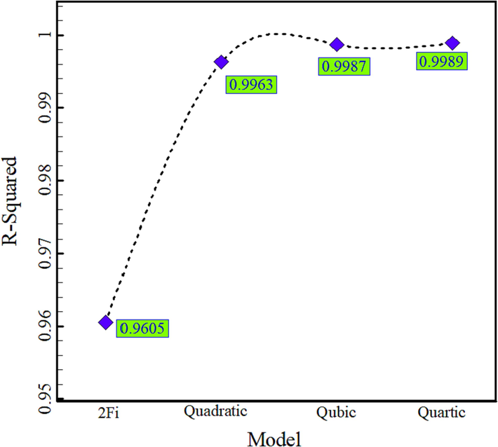
Determination coefficient for 4 different models.
2.2.4 Coefficient of variation parameter
One of the statistical criteria to determine the quality of the model is the coefficient of variation (C.V%). The lower the C.V value, the higher the accuracy of that model. The degree of reliability depends on the relationship between the input variables and the interaction between them. The value of C.V decreases with the increase in the number of parameters used in a model. Reliability values for four different models are reported in Fig. 5. Lowest and highest values of reliability with values of 1.39 and 8.32 belong to Quartic and 2FI models, respectively. Therefore, Quartic model is more accurate and best model.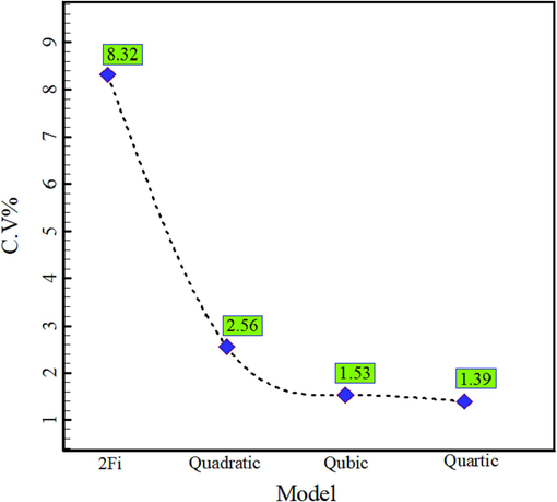
C.V% values for 4 different models.
2.2.5 P-value parameter
P-value means probability or confidence value in statistical methods. P value is used in many statistical methods to check statistical hypotheses. P-value less than 0.05 is used as significance level. In Table 10. P-values for four different models are presented. By comparing four different models, it is clear that the lowest P-value is 8.49355472751e-269 in Quartic model.
Model
P-value
2FI
4.80109569518e-134
Quadratic
3.36147981671e-233
Cubic
5.32248028411e-267
Quartic
8.49355472751e-269
2.3 Model quality determination charts
In this section, the quality of the models and the selection of the best model are discussed using different charts. The graphs that are examined in this section include: predicted values graph versus actual values, normal probability graph, graph of the external studentized residual versus predicted values and Box-Cox graph.
2.3.1 Predicted values versus actual values
In Fig. 6, predicted values of NF viscosity versus actual values of NF viscosity for four different models are presented. In this diagram, the bisector line of 45 degrees is considered as the measurement criterion. If the data is located on bisector line, it has high accuracy model. In Fig. 6, vertical and horizontal axes represent the predicted values of NF viscosity and the actual values of NF viscosity, respectively.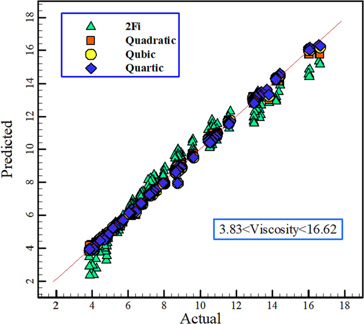
Graph of predicted values of NF viscosity versus actual values of NF viscosity for four different models.
2.3.2 Normal probability diagram
To check whether the data follows a normal distribution or not, a normal probability plot is used. In this diagram, the vertical and horizontal axes show the values of normal probability and the values of external ossified, respectively. In Fig. 7, diagram of normal probability is checked for four models. If the normal probability curve is S-shaped, non-normal data can be converted to normal data using the transfer function. How to recognize the transformation function is determined by the Box-Cox diagram, which will be examined further.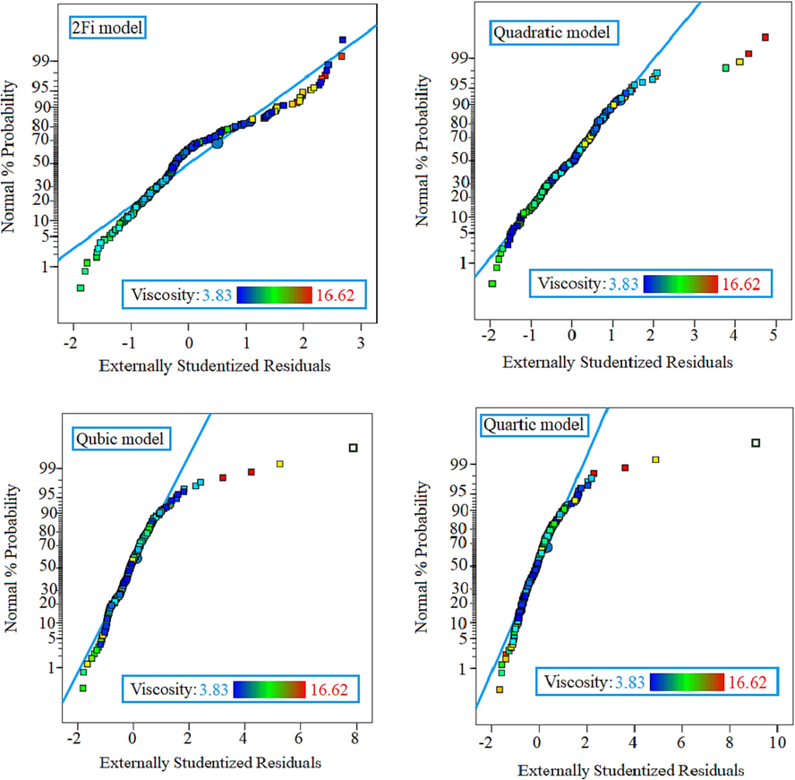
Normal probability plots in four different models.
2.3.3 Externally studentized Residual diagram according to the number of test steps
The externally studentized Residual is a useful tool in regression analysis to detect outliers and evaluate the quality of a model. The main advantage of externally studentized Residual is that they are less sensitive to influential observations in the data set than standard residuals. This means they can be used to detect outliers that may not be detected by other methods. In this diagram, the vertical and horizontal axes show the externally studentized Residual and run number, respectively. Fig. 8 shows the externally studentized Residual for 4 different models.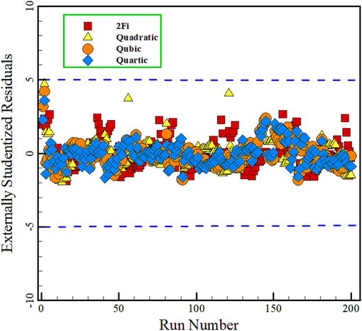
Diagram of externally studentized Residual versus run number for 4 different models.
2.3.4 Box-Cox chart
Box-Cox curve is an analytical tool in the field of statistics to improve the distribution of data and transform them into a normal distribution. Using Box-Cox transformation purpose is improving of data distribution and increase the accuracy of statistical analysis. Having a normal distribution, we can build statistical models more accurately and check the analysis results better. Box-Cox diagram for four models is displayed in Fig. 9. The lowest part of the Box-Cox diagram represents the best value of lambda.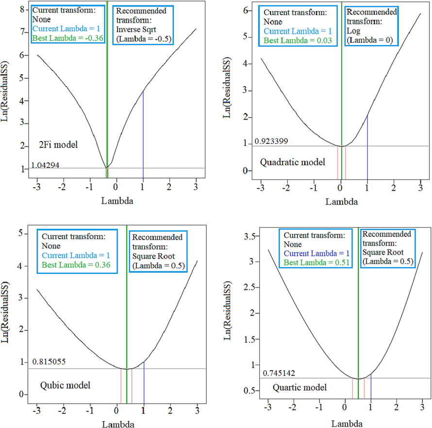
Box-Cox curve of four models.
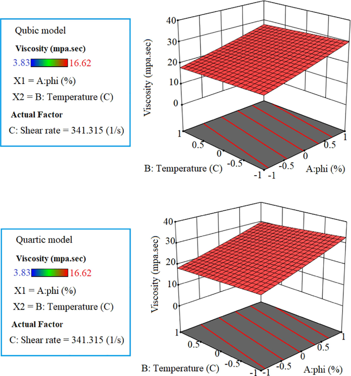
2.3.5 How NF viscosity changes
NF viscosity change according to input variables (SR, SVF and T) for different models is shown in Fig. 10. Decreasing of T and increasing of SVF leads to increasing of NF viscosity. From the comparison of 4 different models, it can be seen that at the same temperature and SVF, the Quartic model shows a higher viscosity value.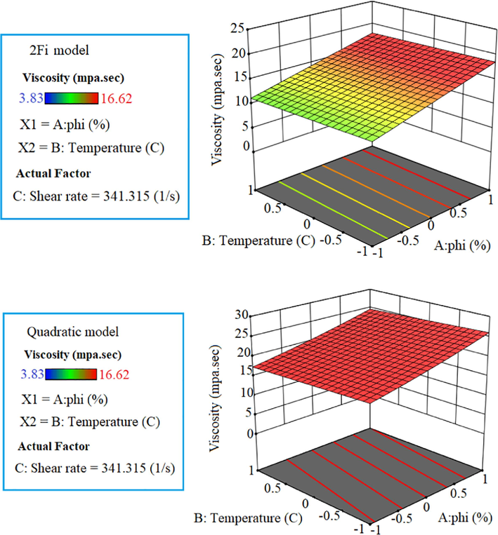
The change trend of NF viscosity for 4 different models.
The change trend of NF viscosity for 4 different models.
2.4 Optimizing the NF viscosity
In this section, CuO NPs dynamic viscosity optimization in EG-Water BF is discussed using the selected model (Quartic model). This study was carried out in cold environmental conditions and according to the restrictions applied in Table 11. In Table 11, values of temperature, SR, SVF and NF viscosity are considered as minimum values. SVF is considered minimum value because of economic efficiency, and because study takes place in a cold environment, therefore, the NF viscosity is considered the minimum value until the engine is turned on; Spraying on parts should happen in the shortest possible time and avoid possible damage such as corrosion and wear. In Table 12, the best lubrication responses for cold environmental conditions are presented. According to Table 12, under conditions of T = 25.303 °C, SVF = 0.05 % and SR = 26.660 s -1, most optimal NF viscosity was obtained 8.565 mPa.sec.
Name
Goal
Lower Limit
Upper Limit
Lower Weight
Upper Weight
Importance
A:
minimize
0.05
1
1
1
3
B:
minimize
15
50
1
1
3
C:
minimize
26.66
933.1
1
1
3
minimize
3.83
16.62
1
1
3
Number
Desirability
1
0.050
25.303
26.660
8.565
0.816
Selected
2
0.050
25.313
26.660
8.561
0.816
3
0.050
25.306
26.661
8.564
0.816
4
0.050
25.298
26.660
8.567
0.816
5
0.050
25.309
26.662
8.563
0.816
6
0.050
25.337
26.661
8.554
0.816
7
0.050
25.331
26.661
8.556
0.816
8
0.050
25.321
26.662
8.559
0.816
9
0.050
25.304
26.661
8.564
0.816
10
0.050
25.298
26.661
8.566
0.816
11
0.050
25.298
26.661
8.567
0.816
12
0.050
25.319
26.662
8.560
0.816
13
0.050
25.302
26.663
8.565
0.816
14
0.050
25.349
26.661
8.550
0.816
15
0.050
25.298
26.663
8.566
0.816
16
0.050
25.326
26.662
8.557
0.816
17
0.050
25.315
26.661
8.561
0.816
18
0.050
25.336
26.661
8.554
0.816
19
0.050
25.301
26.660
8.565
0.816
20
0.050
25.278
26.660
8.573
0.816
In Fig. 11, graphs of NF viscosity and desirability based on changes in temperature and SVF are presented. As can be seen, decreasing T and increasing SVF result to increasing of NF viscosity. According to Fig. 11 and Table 12, the approval rate for the proposed proposal was 81.6 %, which is an acceptable percentage.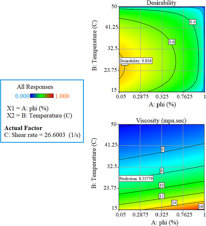
Graphs of NF viscosity and desirability based on changes in T and SVF.
3 Conclusion
In this study, various types of correlation relations were investigated by different models to predict the dynamic viscosity of CuO NPs in EG-Water BF using RSM. Quadratic, Cubic, 2FI and Quartic models have been investigated. These four different models were analyzed based on the measurement criteria. Among these four models, the Quartic model have been chosen as superior model and used to optimize NF viscosity. The optimization was done in cold environmental and variables of SR, SVF, T and viscosity were selected as minimum values and applied to the system. The most important results of this study include the following:
-
Based on the measurement criteria, the Quartic model has been chosen as best model that had higher accuracy than other models.
-
The high coefficient of determination in Quartic model (R2 = 0.9989) with compared to other models causes the percentage of influence and interaction of input variables to be higher.
-
The repeatability percentage of Quartic model is higher than other models due to the low C.V in this model (C.V = 1.39 %).
-
Quartic model is more accurate than other models from the comparison of P-values in four models. (P-value = 8.49355472751e-269).
-
According to the examination of the correlation deviation for four models, Quartic model has less error in predicting the data. (-9.25714 < C.D%<2.34869).
-
At T = 25.303 °C, SVF = 0.05 % and SR = 26.660 sec-1, the most optimal NF viscosity value is 8.565 mPa.sec.
Declaration of competing interest
The authors declare that they have no known competing financial interests or personal relationships that could have appeared to influence the work reported in this paper.
References
- Comparing various machine learning approaches in modeling the dynamic viscosity of CuO/water nanofluid. J. Therm. Anal. Calorim.. 2020;139:2585-2599.
- [Google Scholar]
- Evaluation of the effects of the presence of ZnO -TiO2 (50 %–50 %) on the thermal conductivity of Ethylene Glycol base fluid and its estimation using Artificial Neural Network for industrial and commercial applications. J. Saudi Chem. Soc.. 2023;27(2):101613
- [CrossRef] [Google Scholar]
- Thermal conductivity and viscosity: Review and optimization of effects of nanoparticles. Materials. 2021;14(5):1291.
- [Google Scholar]
- An updated review on application of nanofluids in flat tubes radiators for improving cooling performance. Renew. Sustain. Energy Rev.. 2020;134:110242
- [Google Scholar]
- An experimental study on characterization, stability and dynamic viscosity of CuO-TiO2/water hybrid nanofluid. J. Mol. Liq.. 2020;307:112987
- [Google Scholar]
- Choi, S. U., & Eastman, J. A. (1995). Enhancing thermal conductivity of fluids with nanoparticles (No. ANL/MSD/CP-84938; CONF-951135-29). Argonne National Lab.(ANL), Argonne, IL (United States).
- Using Gaussian Process Regression (GPR) models with the Matérn covariance function to predict the dynamic viscosity and torque of SiO2/Ethylene glycol nanofluid: A machine learning approach. Eng. Appl. Artif. Intel.. 2023;122(106107):106107
- [Google Scholar]
- Experimental study on the thermal conductivity and viscosity of ethylene glycol-based nanofluid containing diamond–silver hybrid material. Diam. Relat. Mater.. 2019;96:216-230.
- [Google Scholar]
- Computational Simulation of Heat Transfer Enhancement in Heat Exchanger Using TiO₂ Nanofluid. J. Complex Flow. 2021;3(2):1-6.
- [Google Scholar]
- An experimental determination and accurate prediction of dynamic viscosity of MWCNT (% 40)-SiO2 (% 60)/5W50 nano-lubricant. J. Mol. Liq.. 2018;259:227-237.
- [Google Scholar]
- Investigation of rheological behavior of hybrid oil based nanolubricant-coolant applied in car engines and cooling equipments. Appl. Therm. Eng.. 2018;131:1026-1033.
- [Google Scholar]
- Experimental investigation of switchable behavior of CuO-MWCNT (85%–15%)/10W-40 hybrid nano-lubricants for applications in internal combustion engines. J. Mol. Liq.. 2017;242:326-335.
- [Google Scholar]
- Experimental study for developing an accurate model to predict viscosity of CuO–ethylene glycol nanofluid using genetic algorithm based neural network. Powder Technol.. 2018;338:383-390.
- [Google Scholar]
- A well-trained artificial neural network (ANN) using the trainlm algorithm for predicting the rheological behavior of water–Ethylene glycol/WO3–MWCNTs nanofluid. Int. Commun. Heat Mass Transfer. 2022;131:105857
- [Google Scholar]
- Experimental investigation of the effects of temperature and mass fraction on the dynamic viscosity of CuO-paraffin nanofluid. Appl. Therm. Eng.. 2018;128:189-197.
- [Google Scholar]
- A new correlation for estimating the thermal conductivity and dynamic viscosity of CuO/liquid paraffin nanofluid using neural network method. Int. Commun. Heat Mass Transfer. 2018;92:90-99.
- [Google Scholar]
- Numerical and experimental evaluation of nanofluids based photovoltaic/thermal systems in Oman: Using silicone-carbide nanoparticles with water-ethylene glycol mixture. Case Stud. Therm. Eng.. 2021;26:101009
- [Google Scholar]
- Experimental investigation of enhanced heat transfer of a car radiator using ZnO nanoparticles in H2O–ethylene glycol mixture. J. Therm. Anal. Calorim.. 2019;138(5):3007-3021.
- [Google Scholar]
- Competition of ANN and RSM techniques in predicting the behavior of the CuO-liquid paraffin. Chem. Eng. Commun. 2021:1-13.
- [Google Scholar]
- Effect of aggregation on the viscosity of copper oxide–gear oil nanofluids. Int. J. Therm. Sci.. 2011;50(9):1741-1747.
- [Google Scholar]
- Heat transfer studies on ethylene glycol/water nanofluid containing TiO2 nanoparticles. Int. J. Refrig. 2019;102:55-61.
- [Google Scholar]
- Stability, thermal performance and artificial neural network modeling of viscosity and thermal conductivity of Al2O3-ethylene glycol nanofluids. Powder Technol.. 2020;363:360-368.
- [Google Scholar]
- Forced convection heat transfer of nanofluids in turbulent flow in a flat tube of an automobile radiator. Energy Rep.. 2022;8:1185-1195.
- [Google Scholar]
- Effects of multi walled carbon nanotubes shape and size on thermal conductivity and viscosity of nanofluids. Diam. Relat. Mater.. 2019;93:96-104.
- [Google Scholar]
- An updated review on application of nanofluids in heat exchangers for saving energy. Energ. Conver. Manage.. 2019;198:111886
- [Google Scholar]
- Experimental investigation of thermo-physical properties of tri-hybrid nanoparticles in water-ethylene glycol mixture. Walailak J. Sci. Technol. (WJST). 2021;18(8):9335-19315.
- [Google Scholar]
- Stability and thermal conductivity of tri-hybrid nanofluids for high concentration in water-ethylene glycol (60: 40) Nanosci. Nanotechnol. Asia. 2021;11(4):121-131.
- [Google Scholar]
- Statistical modeling and investigation of thermal characteristics of a new nanofluid containing cerium oxide powder. Heliyon. 2022;8(11):e11373.
- [Google Scholar]
- A Comprehensive Review on Thermal Conductivity and Viscosity of Nanofluids. J. Adv. Res. Fluid Mech. Therm. Sci.. 2022;91(2):15-40.
- [Google Scholar]
- Functionalized graphene nanoplatelet nanofluids based on a commercial industrial antifreeze for the thermal performance enhancement of wind turbines. Appl. Therm. Eng.. 2019;152:113-125.
- [Google Scholar]
- Nanofluids: Key parameters to enhance thermal conductivity and its applications. Appl. Therm. Eng.. 2022;118202
- [Google Scholar]


