

Translate this page into:
QSAR models for prediction study of HIV protease inhibitors using support vector machines, neural networks and multiple linear regression
⁎Corresponding author.
-
Received: ,
Accepted: ,
This article was originally published by Elsevier and was migrated to Scientific Scholar after the change of Publisher.
Peer review under responsibility of King Saud University.

Abstract
Support vector machines (SVM) represent one of the most promising Machine Learning (ML) tools that can be applied to develop a predictive quantitative structure–activity relationship (QSAR) models using molecular descriptors. Multiple linear regression (MLR) and artificial neural networks (ANNs) were also utilized to construct quantitative linear and non linear models to compare with the results obtained by SVM. The prediction results are in good agreement with the experimental value of HIV activity; also, the results reveal the superiority of the SVM over MLR and ANN model. The contribution of each descriptor to the structure–activity relationships was evaluated.
Keywords
QSAR
HIV protease inhibitors
Support vector machines
Neural networks

1 Introduction
Quantitative structure–activity relationship (QSAR) is a mathematical model of activity in terms of structural descriptors. The QSAR model is useful for understanding the factors controlling activity and for designing new potent compounds (Hasegawa et al., 1996). The main problems encountered in this kind of research are still the description of the molecular structure using appropriate molecular descriptors and selection of suitable modeling methods. At present, many types of molecular descriptors such as topological indices and quantum chemical parameters have been proposed to describe the structural features of molecules (Karelson, 2000; Devillers and Balaban, 1999; Todeschini and Consonni, 2000). Many different chemometric methods, such as multiple linear regression (MLR), partial least squares regression (PLS), different types of neural networks (NNs), genetic algorithms (GAs), and support vector machine (SVM) can be employed to derive correlation models between the molecular structures and properties.
As a new and powerful modeling tool, support vector machine (SVM) has gained much interest in pattern recognition and function approximation applications recently. In bioinformatics, SVMs have been successfully used to solve classification and correlation problems, such as cancer diagnosis (Sweilam et al., 2010; Chen et al., 2011), identification of HIV protease cleavage sites (Wentong and Xuefeng, 2009; Lumini and Nanni, 2006; Noslen et al., 2009), and protein class prediction (Hua and Sun, 2001). SVMs have also been applied in chemistry, for example, the prediction of retention index of protein, and other QSAR studies (Tugcu et al., 2003; Kramer et al., 2002; Warmuth et al., 2003; Liu et al., 2003; Hua et al., 2009; Darnag et al., 2010, 2009; Ivanciuc, 2002; Song et al., 2002; Burbidge et al., 2001). Compared with traditional regression and neural network methods, SVMs have some advantages, including global optimum, good generalization ability, simple implementation, few free parameters, and dimensional independence (Vapnik, 1998; Scholkopf and Smola, 2002). The flexibility in regression and ability to approximate continuous function make SVMs very suitable for QSAR studies.
HIV protease, encoded by human immunodeficiency virus (HIV), plays a very important role during the HIV life cycle. The mature and infectious viral particles can only be generated when the precursor polyproteins are cleaved by the HIV protease properly; otherwise, the viral particles are inactive (Graves et al., 1992). Accordingly, HIV protease has been considered to be a promising target for the rational design of drugs against acquired immunodeficiency syndrome (AIDS). Actually, many effects have been made to understand the specificity of HIV protease and to design HIV protease inhibitors (Chou, 1996). HIV protease is one of the major viral targets for the development of new chemotherapeutics. Currently, many HIV protease inhibitors are used in combination with HIV reverse transcriptase inhibitors. In the present paper, we present the applications of Support Vector Regression (SVR) to investigate the relationship between structure and activity of 38 cyclic-urea derivatives, inhibiting HIV protease based on molecular descriptors. The performance and predictive capability of support vector machine method are investigated and compared with other methods such as artificial neural network and multiple linear regression methods. Thereafter, we sought to measure the contribution of each molecular descriptor.
2 Materials and computer methods
2.1 Data set
In QSAR studies, compounds must be represented using molecular descriptors. A wide variety of descriptors have been reported for QSAR analysis, such as topological, geometrical, electrostatic and quantum chemical descriptors.
The set of 38 cyclic-urea derivatives, inhibiting HIV protease was compiled from the literature (Garg et al., 1999). The HIV protease inhibitor activity (Ki in nM) data of cyclic-urea derivatives were taken from the published work of Garg et al. (1999). The Ki values were converted into the negative logarithmic scale (log(1/Ki)). The log(1/Ki) values were used as response variables. The activities of compounds are shown in Table 1. All the molecules studied had the same parent skeleton (Fig. 1). Each molecule is described by a vector whose elements are parameters measuring physical factors that we considered important for protein–inhibitor interaction, in our study, each molecule was described by four descriptors
-
The indicator variables, Ia = 1 stands for an R/R′ substituent containing an aromatic moiety and Io = 1 stands for an ortho substituent in the aromatic moiety.
-
Charge: dipole moment Δ.
-
MgVol: the molar volume calculated by using the method of McGowan.
| No. | Substituents | log(1/Ki) | |||
|---|---|---|---|---|---|
| R/R′ | Expc | MLRd | ANNe | SVMf | |
| 1 | CH2C6H5(A)a | 8.47 | 8.30 | 8.52 | 8.23 |
| 2 | Me(A) | 5.30 | 6.00 | 5.63 | 5.65 |
| 3 | CH2C6H4-4-CHMe2(A) | 8.96 | 9.96 | 8.76 | 9.12 |
| 4 | CH2C6H4-4-CHMe2(A) | 8.47 | 8.44 | 8.49 | 8.46 |
| 5g | CH2CHMe2(A) | 5.77 | 5.34 | 6.46 | 5.54 |
| 6 | CH(Me)SMe(A) | 5.96 | 5.59 | 5.40 | 5.71 |
| 7 | CH2-3-indolyl(A)a | 6.24 | 6.17 | 6.32 | 6.22 |
| 8 | CH2-Cy-C6H11(A)a | 7.55 | 6.97 | 6.37 | 7.30 |
| 9 | CH2CH2C6H5(A)a | 6.50 | 6.37 | 6.41 | 6.39 |
| 10 | CH2-2-naphthyl(A) | 8.01 | 8.97 | 8.06 | 8.13 |
| 11g | CH2-3-furanyl(A) | 8.08 | 8.53 | 8.05 | 7.89 |
| 12 | CH2C6H4-3-SMe(A) | 8.60 | 8.56 | 8.60 | 8.59 |
| 13 | CH2C6H4-4-SO2Me-(A) | 8.60 | 9.74 | 8.63 | 8.79 |
| 14g | CH2C6H4-2-OMe-(A) | 7.22 | 7.28 | 7.08 | 7.59 |
| 15 | CH2C6H4-2-OH(A) | 7.46 | 8.46 | 8.08 | 7.71 |
| 16 | CH2C6H4-3-OMe(A) | 8.33 | 8.90 | 8.36 | 8.20 |
| 17g | CH2C6H4-4-OMe(A) | 8.07 | 7.24 | 7.95 | 7.95 |
| 18 | CH2C6H4-4-OH(A) | 8.96 | 8.77 | 8.80 | 8.71 |
| 19 | CH2C6H4-3-NH2(A) | 8.55 | 8.38 | 8.55 | 8.34 |
| 20 | CH2C6H4-3-NMe2(A) | 8.37 | 8.44 | 8.42 | 8.49 |
| 21 | CH2C6H4-4-NH2(A) | 8.07 | 7.90 | 8.08 | 7.87 |
| 22g | C6H4-4-NH2-2HCl(A) | 8.15 | 7.98 | 7.98 | 7.95 |
| 23 | CH2C6H4-4-NMe2(A) | 7.34 | 7.43 | 7.08 | 7.50 |
| 24 | CH2-4-pyridyl(A) | 7.66 | 8.51 | 7.57 | 7.44 |
| 25 | 3-(2,5-Me-pyrolyl)-CH2C6H4(A) | 6.80 | 7.79 | 6.90 | 7.92 |
| 26 | CH2C6H4-3,4-(-OCH2O-)(A) | 8.89 | 8.71 | 8.72 | 8.69 |
| 27 | CH2C6H5(B)b | 8.72 | 8.82 | 8.72 | 8.61 |
| 28g | CH2CHMe2(B) | 7.07 | 7.15 | 6.74 | 7.02 |
| 29 | CHMe2(B) | 6.60 | 7.09 | 5.86 | 6.85 |
| 30 | CH(Me)SMe(B) | 5.60 | 5.96 | 5.55 | 5.64 |
| 31 | CH2C6H4-4-F(B) | 8.24 | 8.92 | 8.35 | 8.13 |
| 32g | CH2C6H4-2-OMe(B) | 7.19 | 7.25 | 7.23 | 7.46 |
| 33 | CH2C6H4-3-OMe(B) | 9.06 | 8.92 | 8.84 | 8.79 |
| 34 | CH2C6H4-3-OH(B) | 7.89 | 7.91 | 7.81 | 7.75 |
| 35g | CH2C6H4-4-OMe(B) | 8.54 | 8.41 | 8.05 | 8.30 |
| 36 | CH2-naphthyl(B) | 8.37 | 8.19 | 8.38 | 8.15 |
| 37 | CH2C6H3-3,5-OMe(B) | 8.57 | 8.39 | 8.58 | 8.36 |
| 38 | CH2-2-thienyl(B) | 8.04 | 8.29 | 8.22 | 8.06 |
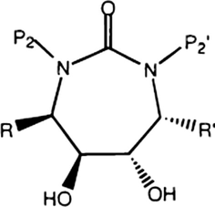
- Chemical formulae of the inhibitors.
2.2 Chemometric methods
2.2.1 Multiple linear regression
MLR is a statistical tool that regresses independent variables against a dependent variable. The objective of MLR is to find a linear model of the property of interest, which takes the form below: where y is the property which is the dependent variable, xi represents molecular descriptors, ai represents the coefficients of those descriptors and α0 is the intercept of the equation.
2.2.2 Artificial neural networks
ANNs are artificial systems simulating the function of the human brain. Three components constitute a neural network: the processing elements or nodes, the topology of the connections between the nodes, and the learning rule by which new information is encoded in the network. While there are a number of different ANN models, the most frequently used type of ANN in QSAR is the three-layered feed-forward network (Zupan and Gasteiger, 1993). In this type of networks, the neurons are arranged in layers (an input layer, one hidden layer and an output layer). Each neuron in any layer is fully connected with the neurons of a succeeding layer and no connections are between neurons belonging to the same layer.
According to the supervised learning adopted, the networks are taught by giving them examples of input patterns and the corresponding target outputs. Through an iterative process, the connection weights are modified until the network gives the desired results for the training set of data. A back-propagation algorithm is used to minimize the error function. This algorithm has been described previously with a simple example of application (Cherqaoui and Villemin, 1994) and a detail of this algorithm is given elsewhere (Freeman and Skapura, 1991).
2.2.3 Support vector machine
SVM is gaining popularity due to many attractive features and promising empirical performance. It originated from early concepts developed by Cortes and Vapnik (1995). This method has proven to be very effective for addressing general purpose classification and regression problems. The main advantage of SVM is that it adopts the structure risk minimization (SRM) principle, which has been shown to be superior to the traditional empirical risk minimization (ERM) principle (Burges, 1998), employed by conventional neural networks. SRM minimizes an upper bound of the generalization error on Vapnik–Chernoverkis dimension (“generalization error”), as opposed to ERM that minimizes the training error. So SVM is usually less vulnerable to the overfitting problem. Since various introductions into SVM were already stated before (Cristianini and Shawe-Taylor, 2000), only the main ideas about SVM are given in this paper.
SVM can be applied to regression problems by the introduction of an alternative loss function that is modified to include a distance measure. Considering the problem of approximating the set of data
(xi is the input vector, di is the desired value, and n is the total number of data patterns). In SVM method, the regression function is approximated, in a feature space F, by the following function:
In Eq. (2), the first term
is called regularized term. Minimizing
will make a function as flat as possible, thus playing role of controlling the function capacity. The second term is the empirical error measured by the ε-insensitive loss function, which is defined by Eq. (3). This defines a ε tube so that if predicted value is within the tube, the loss is zero, while if predicted point is outside the tube, the loss is the magnitude of the difference between the predicted value and the radius ε of the tube. C is penalty parameter, which is a regularized constant to determine the trade-off between training error and model flatness. To get the estimations of w and b, Eq. (2) is transformed into the primal objective Eq. (4) by introducing ξi and
(slack variables representing upper and lower constraints on the outputs of the system).
In Eq. (6), αi and
are the introduced Lagrange multipliers. They satisfy the equality
αi ⩾ 0,
(i = 1, …, n) and are obtained by maximizing the dual form of Eq. (4) which has the following form:
Through selecting the appropriate kernel function, the non-linear relation between the building cooling load and its correlative influence parameters based on SVM is established.
Any function satisfying Mercer’s (1909) condition can be used as the kernel function, and the typical kernel functions include linear, polynomial, Gaussian and sigmoid functions. Among these functions, the Gaussian function can map the sample set from the input space into a high dimensional feature space effectively, which is good for representing the complex non-linear relationship between the output and input samples. Moreover, there is only one variable (the width parameter) in it needed to be determined, which ensures the high calculation efficiency. Because of the above advantages, the Gaussian function is used widely. In this paper, Gaussian function is also selected as the kernel function, whose expression is shown as follows:
All SVM models, in our present study, were implemented using the software LIBSVM for classification and regression developed by Chang and Lin. All calculation programs implementing ANN were written in an M-file based on the MATLAB script, developed in our laboratory.
2.3 Model development
The original data set (38 compounds) was split into a training set (30 compounds), used for establishing the QSAR models and selecting the parameters of the methods used, and a test set (eight compounds) for external validation. The test set is selected such that each of its members is close to at least one point of the training set. To assess the predictivity of the developed QSAR models, several diagnostic statistical tools are used:
2.3.1 Root Mean Square Error (RMSE)
The residual between observed and estimated data is evaluated. This index assumes that larger estimated errors are of greater importance than smaller ones; hence they are given a more than proportionate penalty. The RMSE is known to be descriptive when the prediction capability among predictors is compared, it is defined by:
2.3.2 Scatter Index (SI)
SI is a standard metric for wave model intercomparison. Essentially, it is a normalized measure of error that takes into account the observed data. It is defined as:
Lower values of the SI are an indication of a better prediction.
2.3.3 Correlation coefficient
The predictive power of the QSAR models developed on the selected training sets is estimated on the predictions of an external test set and also examined by cross validation test to the calculating statistical parameters of Q2:
2.3.4 Average Absolute Relative Error (AARE)
AARE indicates the relative absolute deviation in percent from the experimental values. It is defined as:
A lower value implies a better correlation.
In these equations, ym is the desired output, is the predicted value by model, is the mean of dependent variable, and N is the number of the molecules in data set.
3 Results and discussion
In order to develop QSAR models for predicting the biological activity of cyclic-urea derivatives, inhibiting HIV protease, the most commonly practiced stages (optimization, prediction model development and the descriptor's contribution) have been achieved: The first one was aimed at selecting the parameters of the MLR, ANN and SVM. The second one was aimed at determining the predictive ability of these methods. In the third session, we attempt an evaluation of the importance of the descriptors used.
3.1 Optimization
The training set (30 compounds) is used to select the parameters of SVM, ANN and MLR methods.
3.1.1 Support vector machine
The training of the SVM model included the selection of capacity parameter C, ε of ε-insensitive loss function and the corresponding parameters of the kernel function. Firstly, the kernel function should be decided, which determines the sample distribution in the mapping space. Generally, using RBF kernel function will yield better prediction performance (Nianyi et al., 2004), and it was used as the SVM model's kernel in this study accordingly. The radial basis function used is: where γ is the parameter of the kernel, μ and ν are two independent variables.
Secondly, corresponding parameters, i.e., γ of the kernel function greatly affects the number of support vectors, which has a close relation with the performance of the SVM and training time. Over many support vectors could produce overfitting and increase the training time. In addition, γ controls the amplitude of the RBF function, and therefore, controls the generalization ability of SVM.
Parameter ε-insensitive prevents the entire training set meeting boundary conditions and so allows for the possibility of sparsity in the dual formulation's solution. The optimal value for ε depends on the type of noise present in the data, which is usually unknown.
Lastly, the effect of capacity parameter C was tested. It controls the trade-off between maximizing the margin and minimizing the training error. If C is too small then insufficient stress will be placed on fitting the training data. If C is too large then the algorithm will overfit the training data. However, Wang et al. (2005) indicated that prediction error was scarcely influenced by C. To make the learning process stable, a large value should be set up for C.
The grid optimization of LIBSVM was used to find the optimal values of the C, γ and ε parameters when using the radial basis function kernel in the SVM mode. In the grid for data set, a series of C values ranging from 50 to 600 with incremental steps of 50, γ in the range from 0.005 to 0.05 with incremental steps of 0.005 and ε from 0.05 to 0.5 with incremental steps of 0.05 have been exploited. The optimal values of C, γ and ε are identified to be 150, 0.02 and 0.5, respectively. The values of R2 and RMSE are 0.94 and 0.275, respectively. Because the grid search was performed over three parameters, the RMSE could not be shown in one plot to be visualized easily. Figs. 2a–2c show the influence of each parameter with the other two fixed to the optimal values on the model performance.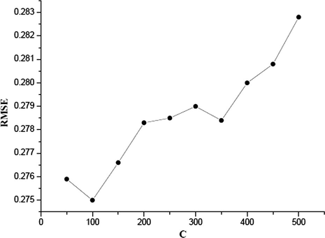
RMSE versus C (γ = 0.01, ε = 0.25).
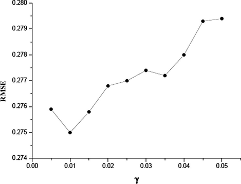
RMSE versus γ (C = 100, ε = 0.25).
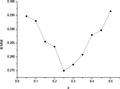
RMSE versus ε (C = 100, γ = 0.01).
3.1.2 Artificial neural networks
All the feed-forward ANNs used in this paper are three-layer networks with 10 units (10 molecular descriptors) in the input layer, a variable number of hidden neurons, and one unit (log(1/Ki)) in the output layer. A bias term was added to the input and hidden layers. Each neuron in any layer is fully connected with the neurons of a succeeding layer. There are neither connections between the neurons within a layer nor any direct connection between those of the input and the output layers. Input and output data are normalized between 0.1 and 0.9. The sigmoid function was used as the transformation function (Freeman and Skapura, 1991). The weights of the connections between the neurons were initially assigned with random values uniformly distributed between −0.5 and +0.5 and no momentum was added. The learning rate was initially set to 1 and was gradually decreased during training. The back-propagation algorithm was used to adjust those weights.
One major problem in neural network is how to determine the number of nodes in the hidden layer. Though there is no rigorous rule to rely on (Golbraikh and Tropsha, 2002), a practical way is to use a ratio, ρ, to determine the number of hidden units (Andrea and Kalayeh, 1991). ρ is defined as the following:
The reasonable value of ρ should be between 1.0 and 3.0. If ρ < 1, the network simply memorizes the data, whereas if ρ > 3, the network is not able to generalize (Golbraikh and Tropsha, 2002). In our study, the four selected variables were used as input and the analgesic activity was used as output, so a 4-x-1 (x represents the number of hidden neurons) network was constructed and the suitable value of x could be defined from 2 to 5 (ρ was located between 1.0 and 2.5). Each architecture was trained with 10 different initial random sets of weights and with the number of cycles limited to 1000. In all cases 100 cycles were enough to obtain stable results. The results are reported in Table 2. Among all architectures of ANN, the best one is 4-4-1 (R2 = 0.92 and RMSE = 0.319).
ANN architecture
R2
RMSE
SI
4-2-1
0.88
0.358
0.046
4-3-1
0.90
0.333
0.043
4-4-1
0.92
0.319
0.041
4-5-1
0.86
0.384
0.049
3.1.3 Multiple linear regression
The linear function constructed from the four molecular descriptors and the training set has the following form:
3.2 Prediction model development
The main goal of any QSAR modeling is that the developed model should be robust enough to be capable of making accurate and reliable predictions of biological activities of new compounds. Tropsha et al. (2003) emphasize the importance of rigorous validation as a crucial, integral component of QSAR model development. The validation strategies check the reliability of the developed models for their possible application on a new set of data, and confidence of prediction can thus be judged.
For the present work, the proposed methodology was validated using several strategies: internal validation, external validation using division of the entire data set into training and test sets and Y-randomization. Furthermore, the domain of applicability which indicates the area of reliable predictions was defined.
3.2.1 Internal validation
The internal validation technique used is cross-validation (CV). CV is a popular technique used to explore the reliability of statistical models. Based on this technique, a number of modified data sets are created by deleting in each case one or a small group (leave-some-out) of objects. For each data set, an input–output model is developed, based on the utilized modeling technique. The model is evaluated by measuring its accuracy in predicting the responses of the remaining data (the ones that have not been utilized in the development of the model). The leave-one-out (LOO) procedure was utilized, in this study, which produces a number of models by deleting one from the whole data set (38 cyclic-urea derivatives).
Five ANN architectures of 4-x-1 (x = 1–5) have been tested. The results of QSAR done by these ANN architectures, by MLR analysis and by SVM method are listed in Table 3. The quality of the fitting is estimated by the RMSE and by the statistical parameter Q. As it can be seen in Table 3, high correlation coefficient (Q2 = 0.89) and low RMSE = 0.171, SI = 0.022 have been obtained by means of the SVM. According to this table, it is clear that the performance of SVM is better than those obtained by ANN and MLR techniques. Indeed, in every case, the SVM's correlation coefficient is greater and its standard deviation is lower than those of the ANN and MLR.
Method
Q2
RMSE
SI
SVM
0.89
0.171
0.022
ANN
0.83
0.265
0.034
MLR
0.77
0.330
0.043
3.2.2 External validation
In order to estimate the predictive power of SVM, MLR and ANN, we must use a set of compounds which have not been used for training set (used for establishing the QSAR model). The models established in the computation procedure, by using the 30 cyclic-urea derivatives, are used to predict the activity of the remaining eight compounds. The plot of predicted versus experimental values for data set is shown in Fig. 3a (SVM), Fig. 3b (ANN) and Fig. 3c (MLR). Among all these figures, the first one shows that the activity values calculated by the SVM are very close to the experimental ones. The statistical parameters of the three models are shown in Table 4. As can be seen from this table, the statistical parameters of SVM model are better than the other ones.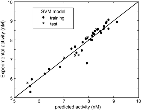
log(1/Ki) observed experimentally versus log(1/Ki) predicted by SVM.
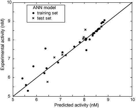
log(1/Ki) observed experimentally versus log(1/Ki) predicted by ANN.
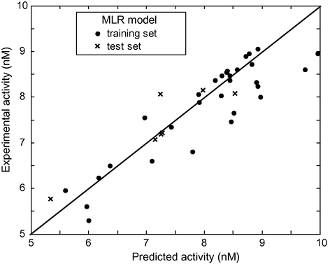
log(1/Ki) observed experimentally versus log(1/Ki) predicted by MLR.
Method
Training set
Test set
R2
ARRE (%)
RMSE
SI
Q2
ARRE (%)
RMSE
SI
SVM
0.94
0.027
0.275
0.035
0.93
0.028
0.227
0.030
ANN
0.92
0.026
0.319
0.041
0.89
0.036
0.334
0.044
MLR
0.81
0.049
0.536
0.069
0.85
0.037
0.377
0.050
3.2.3 Y-randomization test
Y-randomization is an attempt to observe the action of chance in fitting given data. In other words it is applied to exclude the possibility of chance correlation. This technique ensures the robustness of a QSAR model (Tropsha et al., 2003; Tropsha and Golbraikh, 2007). The dependent variable vector [y = log(1/Ki)] is randomly shuffled and a new QSAR model is developed using the original molecular descriptors. The new QSAR models (after several repetitions) are expected to have low R2 values. If the opposite happens then an acceptable QSAR model cannot be obtained for the specific modeling method and data.
In this work, 10 random shuffles of the y vector were performed for SVM, ANN and MLR. The results are shown in Table 5. For each technique, the mean value of random models is significantly lower than the corresponding value of the non-random model. This suggests that the models are not obtained by chance.
Modeling technique
R2 from non random model
Mean value of R2 from model trials
SVM
0.94
0.14
ANN
0.92
0.20
MLR
0.81
0.23
3.2.4 Domain of applicability
The domain of application (Eriksson et al., 2003) of a QSAR model must be defined if the model is to be used for screening new compounds. Predictions for only those compounds that fall into this domain may be considered reliable. Extent of Extrapolation (Gramatica, 2007) is one simple approach to define the applicability of the domain. It is based on the calculation of the leverage hi for each chemical, for which QSAR model is used to predict its activity: where xi is the descriptor vector of the considered compound and X is the descriptor matrix derived from the training set descriptor values. The superscript T refers to the transpose of the matrix/vector. The warning leverage h∗ is, generally, fixed at 3(k + 1)/N, where N is the number of training compounds and k is the number of model parameters. A leverage greater than the warning leverage h∗ means that the predicted response is the result of substantial extrapolation of the model and, therefore, may not be reliable.
The Williams plot for the presented SVM model is shown in Fig. 4. From this plot, the applicability domain is established inside a squared area within (±3s) standard deviations and a leverage threshold h∗ of 0.5. As shown in the Williams plot (Fig. 4), hi values of all the compounds in the training and test sets are lower than the warning value (h∗ = 0.5). None of the compounds are particularly influential in the model space and the training set has great representativeness. For all the compounds in the training and test sets, their standardized residuals are smaller than three standard deviation units (2s). This means that all predicted values are acceptable.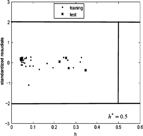
Williams plot of the current QSAR model.
3.3 Analysis of descriptor's contribution
One of the major goals of QSAR studies is the determination of the factors influencing the activity of the studied compounds. They contribute to the comprehension of modes of action composed on their biological targets and guide the synthesis toward compounds with optimal activity. We thus saw necessary to evaluate their contribution of the molecular descriptors to the model established by the SVM. The contribution of each descriptor to the establishment of the QSAR was estimated from the trained SVM using a technique proposed by Cherqaoui et al. (1998). We excluded descriptor i from data set and retrained the resulting SVM as usual. The mean of the deviations' absolute values Δei between the experimental activity and the estimated activity for all compounds has been calculated. This process has been reiterated for each descriptor. Finally, the contribution (Ci) of the descriptor i is given by where N is the number of descriptors.
Fig. 5 indicates that the relative importance of the descriptors varied in the following order: MgVol > Δ > Io > Ia.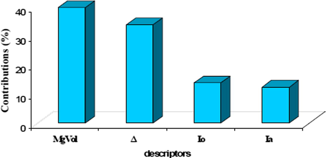
Contributions of the four molecular descriptors to QSAR.
We can notice that the descriptor related to the molar volume calculated by using the method of McGowan (MgVol) and dipole moment (Δ) are the most important in the establishment of the QSAR of cyclic-area derivatives.
4 Conclusion
In the present work, we have compared the performance of MLR, ANN, and SVM in QSAR study. The obtained results show that SVM can be used to derive statistical models with better qualities and better generalization capabilities than linear regression methods. The optimization process of SVM is relatively easy to be implemented. They can be used as alternative nonlinear modeling tools in QSAR. The main factors controlling the biological activity of cyclic-urea derivatives have been determined by SVM. Molar volume and dipole moment parameters of the compounds were thus found to take the most relevant part in the molecular description. The SVM approach would seem to have great potential for determining quantitative structure–HIV-1 activity relationships and as such be a valuable tool for the chemist.
References
- Drug design by machine learning: support vector machines for pharmaceutical data analysis. Comput. Chem.. 2001;26:5-14.
- [Google Scholar]
- A tutorial on support vector machines for pattern recognition. Data Min. Knowl. Discov.. 1998;2:121-167.
- [Google Scholar]
- Chang, C.C., Lin, C.J. LIBSVM – a library for support vector machine. <http://www/csie.edu/tw/cjlin/libs/libsvm>.
- A support vector machine classifier with rough set-based feature selection for breast cancer diagnosis. Expert Syst. Appl.. 2011;38:9014-9022.
- [Google Scholar]
- Use of neural network to determine the boiling point of alkanes. J. Chem. Soc. Faraday Trans.. 1994;90:97-102.
- [Google Scholar]
- Structure musk odour relationships studies of tetralin and indan compounds using neural networks. New J. Chem.. 1998;22:839-843.
- [Google Scholar]
- Prediction of HIV protease cleavage sites in proteins. Anal. Biochem.. 1996;233:1-14.
- [Google Scholar]
- An Introduction to Support Vector Machines. Cambridge, UK: Cambridge University Press; 2000.
- QSAR studies of HEPT derivatives using support vector machines. QSAR Comb. Sci.. 2009;28:709-718.
- [Google Scholar]
- Support vector machines: development of QSAR models for predicting anti-HIV-1 activity of TIBO derivatives. Eur. J. Med. Chem.. 2010;45:1590-1597.
- [Google Scholar]
- Topological Indices and Related Descriptors in QSAR and QSPR. Amsterdam, Netherlands: Gordon and Breach; 1999.
- Methods for reliability and uncertainty assessment and for applicability evaluations of classification- and regression-based QSARs. Environ. Health Perspect.. 2003;111:1361-1375.
- [Google Scholar]
- Neural Networks Algorithms, Applications, and Programming Techniques. Reading: Addition Wesley Publishing Company; 1991.
- Principles of QSAR models validation: internal and external. QSAR Comb. Sci.. 2007;26:694-701.
- [Google Scholar]
- Dunn B., ed. Structure and Function of the Aspartic Protease: Genetics, Structure and Mechanisms. New York: Plenum; 1992.
- Multivariate Free-Wilson analysis of α-chymotrypsin inhibitors using PLS. Chemom. Intell. Lab. Syst.. 1996;33:63-69.
- [Google Scholar]
- Novel method of protein secondary structure prediction with high segment overlap measure: support vector machine approach. J. Mol. Biol.. 2001;308:397-407.
- [Google Scholar]
- QSAR models for 2-amino-6-arylsulfonylbenzonitriles and congeners HIV-1 reverse transcriptase inhibitors based on linear and nonlinear regression methods. Eur. J. Med. Chem.. 2009;44:2158-2171.
- [Google Scholar]
- Support vector machine identification of the aquatic toxicity mechanism of organic compounds. Internet Electron. J. Mol. Des.. 2002;1:151-172.
- [Google Scholar]
- Molecular Descriptors in QSAR/QSPR. New York: John Wiley & Sons; 2000.
- Fragment generation and support vector machines for inducing SARs. SAR QSAR Environ. Res.. 2002;13:509-523.
- [Google Scholar]
- QSAR study of ethyl, 2-[(3-methyl-2,5-dioxo(3-pyrrolinyl))amino]-4-(trifluoromethyl)pyrimidine-5-carboxylate: an inhibitor of AP-1 and NF-B mediated gene expression based on support vector machines. J. Chem. Inf. Comput. Sci.. 2003;43:1288-1296.
- [Google Scholar]
- Machine learning for HIV-1 protease cleavage site prediction. Pattern Recognit. Lett.. 2006;27:1537-1544.
- [Google Scholar]
- Functions of positive and negative type and their connection with the theory of integral equations. Philos. Trans. R. Soc. Lond. Ser. A. 1909;209:415-446.
- [Google Scholar]
- Support Vector Machine in Chemistry. NY: World Scientific Publishing Company; 2004.
- Critical comparative analysis, validation and interpretation of SVM and PLS regression models in a QSAR study on HIV-1 protease inhibitors. Chemom. Intell. Lab. Syst.. 2009;98:65-77.
- [Google Scholar]
- Learning with Kernels. Cambridge, MA: MIT Press; 2002.
- Prediction of protein retention times in anion-exchange chromatography systems using support vector regression. J. Chem. Inf. Comput. Sci.. 2002;42:1347-1357.
- [Google Scholar]
- Support vector machine for diagnosis cancer disease: a comparative study. Egypt. Inf. J.. 2010;11:81-92.
- [Google Scholar]
- Handbook of Molecular Descriptors. Weinheim, Germany: Wiley-VCH; 2000.
- Predictive QSAR modeling workflow, model applicability domains, and virtual screening. Curr. Pharm. Des.. 2007;13:3494-3504.
- [Google Scholar]
- The importance of being earnest: validation is the absolute essential for successful application and interpretation of QSPR models. Quant. Struct.-Act. Relat.. 2003;22:1-9.
- [Google Scholar]
- Prediction of the effect of mobile-phase salt type on protein retention and selectivity in anion exchange systems. Anal. Chem.. 2003;75:3563-3572.
- [Google Scholar]
- Statistical Learning Theory. New York: John Wiley & Sons; 1998.
- Determination of the spread parameter in the Gaussian kernel for classification and regression. Neurocomputing. 2005;55:643-663.
- [Google Scholar]
- Active learning with support vector machines in the drug discovery process. J. Chem. Inf. Comput. Sci.. 2003;43:667-673.
- [Google Scholar]
- Adaptive weighted least square support vector machine regression integrated with outlier detection and its application in QSAR. Chemom. Intell. Lab. Syst.. 2009;98:130-135.
- [Google Scholar]
- Neural Networks for Chemists. An Introduction. Weinheim: VCH Publishers; 1993.


