

QSAR study of the non-peptidic inhibitors of procollagen C-proteinase based on Multiple linear regression, principle component regression, and partial least squares
⁎Corresponding author.
-
Received: ,
Accepted: ,
This article was originally published by Elsevier and was migrated to Scientific Scholar after the change of Publisher.
Peer review under responsibility of King Saud University.
Abstract
The quantitative structure–activity relationship (QSAR) analyses were carried out in a series of novel sulfonamide derivatives as the procollagen C-proteinase inhibitors for treatment of fibrotic conditions. Sphere exclusion method was used to classify data set into categories of train and test set at different radii ranging from 0.9 to 0.5. Multiple linear regression (MLR), principal component regression (PCR) and partial least squares (PLS) were used as the regression methods and stepwise, Genetic algorithm (GA), and simulated annealing (SA) were used as the feature selection methods. Three of the statistically best significant models were chosen from the results for discussion. Model 1 was obtained by MLR–SA methodology at a radius of 1.6. This model with a coefficient of determination (r2) = 0.71 can well predict the real inhibitor activities. Cross-validated q2 of this model, 0.64, indicates good internal predictive power of the model. External validation of the model (pred_r2 = 0.85) showed that the model can well predict activity of novel PCP inhibitors. The model 2 which developed using PLS–SW explains 72% (r2 = 0.72) of the total variance in the training set as well as it has internal (q2) and external (pred_r2) predictive ability of ∼67% and ∼71% respectively. The last developed model by PCR–SA has a correlation coefficient (r2) of 0.68 which can explains 68% of the variance in the observed activity values. In this case internal and external validations are 0.61 and 0.75, respectively. Alignment Independent (AI) and atomic valence connectivity index (chiv) have the greatest effect on the biological activities. Developed models can be useful in designing and synthesis of effective and optimized novel PCP inhibitors which can be used for treatment of fibrotic conditions.
Keywords
Fibrosis
Procollagen C-proteinase inhibitors
QSAR
MLR
PLS
PCR

1 Introduction
Collagen is the most abundant structural protein of the various connective tissues in animals. Despite it helps to maintain the integrity of many tissues via its interactions with cell surfaces, excessive production of collagen leads to pathological conditions (Di Lullo et al., 2002). Fibrosis is characterized by excessive accumulation of extracellular matrix (ECM) proteins in response to chronic stress and injury which cause normal wound healing process goes awry (Williams et al., 2014). Fibrosis can occur in many tissues within the body, such as lungs, heart, skin, bone marrow, and soft tissue (Bestetti et al., 2010; Chaudhuri et al., 2014; Hasselbalch, 2013; Mathisen and Grillo, 1992; Shaffer et al., 2002). Despite advances in medical science, fibrosis still remains a major medical problem which has been estimated to play a causal role in nearly 45% of deaths in the developed world (Wynn, 2004). Currently, there are no adequate therapies for fibrotic conditions. So, identification and design of novel drugs specifically affecting these targets could lead to better drugs which are needed for both systemic and topical applications. Procollagen C-endopeptidase (procollagen C-proteinase (PCP)) is an enzyme which cleavages of the C-terminal propeptide at Ala-Asp in type I and II procollagens and at Arg-Asp in type III (Hojima et al., 1985). Cleavage of the globular C-terminal by this endopeptidase converts soluble pro-collagens into fully formed, insoluble, collagen fibrils. So inhibition of PCP is an interesting target in fibrotic conditions which is expected to disrupt fibril formation and stability, therefore, aid in the treatment of these inflammatory conditions (Dankwardt et al., 2002).
The quantitative structure–activity relationship (QSAR) relates a set of physico-chemical properties or molecular descriptors to a response-variable which could be a biological activity of the chemicals (Hansch et al., 2001). One can obtain a rapid and cost-effective biological activities by QSAR without necessity of performing expensive and time consuming laboratory experiments (Dybdahl et al., 2012). Recently, novel inhibitors of procollagen C-proteinase (PCP) have been synthesized and their structure activity relationship (SAR) has been investigated (Bailey et al., 2008; Dankwardt et al., 2002, 2000; Delaet et al., 2003; Robinson et al., 2003; Turtle et al., 2012), but QSAR studies have not been carried out for PCP inhibitors. According to the above matter, we developed some statistically significant QSAR models for sulfonamide derivatives as PCP inhibitors. The obtained result may be used to further and effective designing novel PCP inhibitors.
2 Materials and method
2.1 Data set and structure optimization
A set of 54 molecules of sulfonamide derivatives as nonpeptidic PCP inhibitors were used for the present QSAR study (Turtle et al., 2012). The chemical structure and biological activities (IC50) of these molecules are shown in the Table 1. The molecules have high structural diversity and the activity range is wide. So this data set is suitable for our QSAR studies. To reduce the skewness of data set, the IC50 values were converted to a logarithmic scale (pIC50 = −log (IC50)). Subsequently pIC50 values were used as the response values in the QSAR studies. The compounds were then subjected to conformational analysis and energy minimization using Montocarlo conformational search with root mean square (RMS) gradient of 0.001 kcal/mol using a Merck Molecular Force Field (MMFF). Montocarlo conformational search method is similar to the random incremental pulse search (RIPS) method that generates a new molecular conformation by randomly perturbing the position of each coordinate of each atom in the molecule. Most stable structure for each compound was generated after energy minimization. Then, optimized geometries and corresponding pIC50 were imported into the VLife MDS 3.5 (Vlife Sciences Technologies Pvt. Ltd. Pune, India) software. Vlife MDS is a complete molecular modeling software which can perform tasks such as QSAR, combinatorial Library generation, pharmacophore, cheminformatics, and docking. The energy-minimized molecules were used for the calculation of the various 2D molecular descriptors (Individual, Chi, ChiV, Path count, ChiChain, ChiVChain, Chainpathcount, Cluster, Pathcluster, Kapa, Element Count, and so on). In addition, alignment independent descriptors were calculated and were added to the descriptor list. A descriptor that is constant for all the molecules will not contribute to QSAR and hence was removed. Training and test set were created by using a sphere exclusion method for choosing uniformly distributed molecules in both sets (Hudson et al., 1996; Zheng and Tropsha, 1999). In the acceptable dissimilarity value or sphere exclusion radius the test set should be interpolative i.e. derived within the min–max range of the train set. Radius values varying from 0.8 to 6 were examined which a radius of 0.9 to 5 had an acceptable dissimilarity value and were used for further analysis.
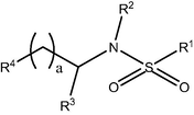
| a | R1 | R2 | R3 | R4 | IC50 (μM) | pIC50 | |
|---|---|---|---|---|---|---|---|
| 1 | 0 | 4-MeO-Ph | H | CH2CO2H | CONHOH | 10.00 | 5.00 |
| 2 | 0 | 4-MeO-Ph | CH2CO2H | H | CONHOH | 345.00 | 3.46 |
| 3 | 0 | 4-MeO-Ph | CH2Ph | H | CONHOH | 16.00 | 4.80 |
| 4 | 0 | 4-MeO-Ph | CH2Ph | CH2CO2H | CONHOH | 2.80 | 5.55 |
| 5 | 0 | 4-MeO-Ph | Ph | H | CONHOH | 69.00 | 4.16 |
| 6 | 0 | 4-MeO-Ph | CH2CH2Ph | H | CONHOH | 18.00 | 4.74 |
| 7 | 1 | 4-MeO-Ph | Ph | H | CONHOH | 3.00 | 5.52 |
| 8 | 1 | 4-MeO-Ph | CH2Ph | H | CONHOH | 4.50 | 5.35 |
| 9 | 1 | 4-MeO-Ph | CH2CH2Ph | H | CONHOH | 0.90 | 6.05 |
| 10 | 2 | 4-MeO-Ph | Ph | H | CONHOH | 28.00 | 4.55 |
| 11 | 2 | 4-MeO-Ph | CH2Ph | H | CONHOH | 10.00 | 5.00 |
| 12 | 2 | 4-MeO-Ph | CH2CH2Ph | H | CONHOH | 4.90 | 5.31 |
| 13 | 0 | 4-MeO-Ph | Sec-butyl | H | CONHOH | 112.00 | 3.95 |
| 14 | 0 | 4-MeO-Ph | CH2(4-F-Ph) | H | CONHOH | 34.00 | 4.47 |
| 15 | 0 | 4-MeO-Ph | CH2CO2n-Bu | H | CONHOH | 167.00 | 3.78 |
| 16 | 0 | 4-MeO-Ph | 4-MeO-Ph | H | CONHOH | 73.00 | 4.14 |
| 17 | 0 | 4-MeO-Ph | CH2CH2(4-MeO)Ph | H | CONHOH | 18.00 | 4.74 |
| 18 | 0 | 4-MeO-Ph | CH2(4-MeO)Ph | H | CONHOH | 29.00 | 4.54 |
| 19 | 0 | 4-MeO-Ph | CH2(4-CF3)Ph | H | CONHOH | 67.00 | 4.17 |
| 20 | 0 | 4-MeO-Ph | CH2(4-Cl)Ph | H | CONHOH | 19.00 | 4.72 |
| 21 | 0 | 4-MeO-Ph | CH(Ph)2 | H | CONHOH | 102.00 | 3.99 |
| 22 | 1 | 4-MeO-Ph | H | H | CONHOH | 81.00 | 4.09 |
| 23 | 1 | 4-MeO-Ph | CH2CH2-N-morpholinyl | H | CONHOH | 1.70 | 5.77 |
| 24 | 1 | 4-MeO-Ph | Sec-butyl | H | CONHOH | 1.00 | 6.00 |
| 25 | 1 | 4-MeO-Ph | CH2-cyclhexane | H | CONHOH | 8.10 | 5.09 |
| 26 | 1 | 4-MeO-Ph | CH2CH2(2-pyridyl) | H | CONHOH | 1.70 | 5.77 |
| 27 | 1 | 4-MeO-Ph | 4-MeO-Ph | H | CONHOH | 1.00 | 6.00 |
| 28 | 1 | 4-MeO-Ph | CH2CH2(4-MeO-Ph) | H | CONHOH | 2.30 | 5.64 |
| 29 | 1 | 4-MeO-Ph | CH2CH2(3-MeO-Ph) | H | CONHOH | 11.00 | 4.96 |
| 30 | 1 | 4-MeO-Ph | CH2CH2(4-NO2-Ph) | H | CONHOH | 23.00 | 4.64 |
| 31 | 1 | 4-MeO-Ph | CH2CH2(4-NH2SO2 -Ph) | H | CONHOH | 42.00 | 4.38 |
| 32 | 1 | 4-MeO-Ph | CH2CH2(3,4-diMeO-Ph) | H | CONHOH | 166.00 | 3.78 |
| 33 | 1 | n-Bu | CH2CH2(4-MeO-Ph) | H | CONHOH | 6.70 | 5.17 |
| 34 | 0 | n-Bu | CH2CH2(4-MeO-Ph) | H | CONHOH | 55.00 | 4.26 |
| 35 | 1 | Ph | CH2CH2Ph | H | CONHOH | 2.20 | 5.66 |
| 36 | 1 | 4-CO2H-Ph | CH2CH2Ph | H | CONHOH | 1.00 | 6.00 |
| 37 | 1 | 4-(C(⚌NOH)NH2)-Ph | CH2CH2(4-MeO-Ph) | H | CONHOH | 0.08 | 7.10 |
| 38 | 1 | 3-(C(⚌NOH)NH2)-Ph | CH2CH2(4-MeO-Ph) | H | CONHOH | 0.40 | 6.40 |
| 39 | 1 | 2-(C(⚌NOH)NH2)-Ph | CH2CH2(4-MeO-Ph) | H | CONHOH | 7.10 | 5.15 |
| 40 | 1 | 4-(Ph-C(⚌O)NH)-Ph | CH2CH2(4-MeO-Ph) | H | CONHOH | 0.41 | 6.39 |
| 41 | 1 | 4-(Ph-SO2-NH)-Ph | CH2CH2(4-MeO-Ph) | H | CONHOH | 0.47 | 6.33 |
| 42 | 1 | 4-SO2Me-Ph | CH2CH2(4-MeO-Ph) | H | CONHOH | 0.29 | 6.54 |
| 43 | 1 | 2-SO2Me-Ph | CH2CH2(4-MeO-Ph) | H | CONHOH | 9.10 | 5.04 |
| 44 | 1 | 4-tBu-Ph | CH2CH2Ph | H | CONHOH | 17.00 | 4.77 |
| 45 | 0 | 4-SO2Me-Ph | CH2CH2(4-MeO-Ph) | H | COCH2SH | 4.70 | 5.33 |
| 46 | 1 | 4-SO2Me-Ph | CH2CH2(4-MeO-Ph) | H | COCH2SH | 13.00 | 4.89 |
| 47 | 2 | 4-SO2Me-Ph | CH2CH2(4-MeO-Ph) | H | SH | 14.00 | 4.85 |
| 48 | 1 | 4-SO2Me-Ph | CH2CH2(4-MeO-Ph) | H | SH | 9.40 | 5.03 |
| 49 | 1 | 4-NHCONHPh-Ph | CH2CH2(4-MeO-Ph) | H | CONHOH | 0.09 | 7.03 |
| 50 | 1 | 4-NHCONH(4-MeO-Ph)-Ph | CH2CH2(4-MeO-Ph) | H | CONHOH | 0.35 | 6.46 |
| 51 | 1 | 4-NHCONH(4-CF3-Ph)-Ph | CH2CH2(4-MeO-Ph) | H | CONHOH | 0.04 | 7.38 |
| 52 | 1 | 4-NHCONH(4-Cl-Ph)-Ph | CH2CH2(4-MeO-Ph) | H | CONHOH | 0.30 | 6.52 |
| 53 | 1 | 4-NHCONHBn-Ph | CH2CH2(4-MeO-Ph) | H | CONHOH | 0.01 | 8.00 |
| 54 | 1 | 4-NHCONHMe-Ph | CH2CH2(4-MeO-Ph) | H | CONHOH | 0.06 | 7.22 |
2.2 Regression and variable selection methods
Feature or variable selection is one of the important steps in a QSAR study, which known as variable selection technique (Guyon and Elisseeff, 2003). In principle, any variable selection method can be coupled with any statistical method of choice for building quantitative model. Multiple linear regression (MLR) (Darlington, 1990), principal component regression (PCR) (Pearson, 1901), and partial least squares (PLS) (Tenenhaus et al., 2005) were used as the regression methods and stepwise, Genetic algorithm (GA), and simulated annealing (SA) were used as the feature selection methods (Metropolis et al., 1953). In the stepwise (SW) feature selection method, forward–backward (FB) was used and the cross-correlation limit was set at 0.5, the number of variables at 5, and the term selection criteria at r2. In the GA method, crosscorrelation limit, population, and number of generations were set at 0.5, 10, and 1000, respectively. In the SA method, maximum temperature, minimum temperature, and crosscorrelation limit were set at 100, 0.01, and 0.5, respectively. At any radius, GA, SA, and FB as the feature selection methods were used with the MLR, PCR and PLS as the regression methods. Variable selection and regressions were done by Vlife MDS software.
2.3 Statistical analysis
The performance of developed QSAR models was evaluated using r2 (the squared correlation coefficient), q2 (cross-validated correlation coefficient), F-test (Fischer’s value) for statistical significance, and pred_r2, (r2 for the external test set). The main utility of a QSAR model is their capability replicated by the model. However, if the following conditions are satisfied a QSAR model will be robust and predictive: r2 > 0.6, q2 > 0.6 and pred_r2 > 0.5 (Golbraikh and Tropsha, 2002). External and internal validation ability of a model is evaluated by some validation criteria. Most important and frequently used criteria are q2 and pred_r2 for internal and external validation, respectively.
2.3.1 Internal validation
The cross-validation analysis was performed using the leave-one-out (LOO) method. Internal or cross-validation criterion (q2) is calculated according to the formula:
2.3.2 External validation
When truly external date points are not available for test of the model prediction ability, original date set are divided into training and test set. The model is built from train set, and then is validated with the test set. pred_r2 is calculated according to the following equation:
where ypred(test) and are ytest predicted and observed activity for test set and
2.3.3 Randomization test
To evaluate the statistical significance of the QSAR model for a real data set, one-tail hypothesis testing was used (Golbraikh and Tropsha, 2003; Gilbert, 1976). To evaluate chance correlation of the models, training sets were examined by comparing these models to those derived from random data sets. Random sets were generated by shuffling the activities of the molecules in the training set. The statistical model was derived using various randomly scrambled activities (random sets) with the selected descriptors and the corresponding q2 values were calculated. The significance of the models, hence obtained was derived based on a calculated Z score (Gilbert, 1976; Cramer et al., 1988). A Z score value is calculated by the following formula:
The probability (α) of significance of randomization test is derived by comparing Z score value with Z score critical value as reported in Table 2 (Shen et al., 2003), if Z score value is less than 4.0; otherwise it is calculated by the formula as given in Table 2. If the Z score is higher than the tabulated values of Zc (Table 2), one concludes that at the level of significance that corresponds to that Zc should be accepted. In this case, it is concluded that the result obtained for the actual data set is statistically much more significant than the results obtained for random data sets at a given level of significance. For example, a Z score value greater than 3.10 indicates that there is a probability (α) of less than 0.001 that the QSAR model constructed for the real data set is random. The randomization test suggests that all the developed models have a probability of less than 1% that the model is generated by chance (Table 3).
| α | Zc |
|---|---|
| 0.10 | 1.28 |
| 0.05 | 1.64 |
| 0.01 | 2.33 |
| 0.001 | 3.10 |
| Regression method | Feature selection method | Radius | ||||||||
|---|---|---|---|---|---|---|---|---|---|---|
| Parameter | 0.9 | 1.6 | 1.7 | 1.9 | 2 | 3 | 4 | 5 | ||
| MLR | Stepwise | r2 | 0.71 | 0.72 | 0.74 | 0.84 | 0.80 | 0.70 | 0.80 | 0.91 |
| q2 | 0.66 | 0.67 | 0.69 | 0.78 | 0.79 | 0.71 | 0.78 | 0.85 | ||
| F-test | 39.45 | 37.37 | 39.28 | 33.94 | 35.71 | 35.59 | 35.66 | 78.83 | ||
| N | 52.00 | 46.00 | 45.00 | 37.00 | 36.00 | 23.00 | 16.00 | 9.00 | ||
| Pred_r2 | 0.96 | 0.69 | 0.47 | 0.37 | 0.17 | 0.36 | 0.29 | −1.48 | ||
| r2 se | 0.56 | 0.57 | 0.55 | 0.46 | 0.47 | 0.61 | 0.55 | 0.42 | ||
| q2 se | 0.61 | 0.62 | 0.60 | 0.54 | 0.56 | 0.69 | 0.65 | 0.55 | ||
| Best rand r2 | 0.26 | 0.28 | 0.22 | 0.33 | 0.44 | 0.34 | 0.42 | 0.92 | ||
| Best rand q2 | 0.14 | 0.14 | 0.06 | 0.11 | 0.17 | 0.18 | 0.10 | 0.86 | ||
| Z score rand r2 | 13.87 | 12.62 | 13.84 | 9.97 | 8.32 | 9.15 | 7.43 | 4.92 | ||
| Z score rand q2 | 12.35 | 10.93 | 11 | 6.14 | 5.81 | 7.98 | 5.44 | 4.24 | ||
| α rand r2 | 0 | 0 | 0 | 0 | 0 | 0 | 0 | 0 | ||
| α rand q2 | 0 | 0 | 0 | 0 | 0 | 0 | 0 | 0 | ||
| Genetic algorithm | r2 | 0.67 | 0.56 | 0.58 | 0.63 | 0.59 | 0.67 | 0.75 | 0.91 | |
| q2 | 0.57 | 0.44 | 0.48 | 0.54 | 0.46 | 0.54 | 0.56 | 0.69 | ||
| F-test | 24.32 | 18.10 | 19.13 | 19.29 | 15.48 | 13.02 | 12.21 | 18.33 | ||
| N | 52.00 | 46.00 | 45.00 | 37.00 | 36.00 | 23.00 | 16.00 | 9.00 | ||
| Pred_r2 | 0.97 | 0.84 | 0.67 | 0.55 | 0.47 | −0.03 | 0.23 | 0.30 | ||
| r2 se | 0.60 | 0.72 | 0.70 | 0.69 | 0.77 | 0.77 | 0.72 | 0.50 | ||
| q2 se | 0.69 | 0.81 | 0.78 | 0.78 | 0.88 | 0.90 | 0.95 | 0.95 | ||
| Best rand r2 | 0.22 | 0.24 | 0.31 | 0.34 | 0.23 | 0.37 | 0.56 | 0.96 | ||
| Best rand q2 | 0.06 | 0.10 | 0.19 | 0.14 | 0.05 | 0.10 | 0.26 | 0.61 | ||
| Z score rand r2 | 12.79 | 9.79 | 9.36 | 9.56 | 9.45 | 6.32 | 4.20 | 2.89 | ||
| Z score rand q2 | 7.89 | 8.11 | 8.19 | 8.15 | 7.30 | 6.48 | 3.96 | 1.81 | ||
| α rand r2 | 0 | 0 | 0 | 0 | 0 | 0 | 0 | 0.01 | ||
| α rand q2 | 0 | 0 | 0 | 0 | 0 | 0 | 0 | 0.05 | ||
| Simulated annealing | r2 | 0.67 | 0.71 | 0.66 | 0.72 | 0.74 | 0.75 | 0.86 | 0.99 | |
| q2 | 0.60 | 0.64 | 0.56 | 0.64 | 0.67 | 0.54 | 0.68 | 0.88 | ||
| F-test | 24.54 | 26.00 | 19.98 | 21.15 | 30.96 | 13.87 | 17.00 | 121.80 | ||
| N | 52.00 | 46.00 | 45.00 | 37.00 | 36.00 | 23.00 | 16.00 | 9.00 | ||
| Pred_r2 | 0.98 | 0.85 | 0.81 | 0.53 | 0.32 | −0.28 | 0.01 | −0.58 | ||
| r2 se | 0.60 | 0.58 | 0.63 | 0.61 | 0.61 | 0.68 | 0.56 | 0.17 | ||
| q2 se | 0.66 | 0.66 | 0.72 | 0.69 | 0.69 | 0.93 | 0.85 | 0.66 | ||
| Best rand r2 | 0.27 | 0.24 | 0.29 | 0.34 | 0.29 | 0.49 | 0.76 | 0.97 | ||
| Best rand q2 | 0.12 | 0.03 | 1.10 | 0.14 | 0.14 | 0.23 | 0.54 | 0.77 | ||
| Z score rand r2 | 11.40 | 11.75 | 9.84 | 8.71 | 11.67 | 4.80 | 3.94 | 2.32 | ||
| Z score rand q2 | 12.15 | 9.41 | 8.13 | 7.52 | 10.02 | 3.12 | 3.48 | 1.92 | ||
| α rand r2 | 0 | 0 | 0 | 0 | 0 | 0 | 0 | 0.05 | ||
| α rand q2 | 0 | 0 | 0 | 0 | 0 | 0 | 0 | 0.05 | ||
| PLS | Stepwise | r2 | 0.70 | 0.72 | 0.74 | 0.84 | 0.85 | 0.77 | 0.78 | 0.91 |
| q2 | 0.65 | 0.67 | 0.68 | 0.78 | 0.79 | 0.71 | 0.72 | 0.85 | ||
| F-test | 57.95 | 57.26 | 59.78 | 43.76 | 46.06 | 74.10 | 51.28 | 78.83 | ||
| N | 52.00 | 46.00 | 45.00 | 37.00 | 36.00 | 23.00 | 16.00 | 9.00 | ||
| Pred_r2 | 0.95 | 0.71 | 0.48 | 0.37 | 0.17 | 0.31 | 0.27 | −1.48 | ||
| r2 se | 0.56 | 0.56 | 0.55 | 0.46 | 0.46 | 0.60 | 0.62 | 0.42 | ||
| q2 se | 0.61 | 0.61 | 0.60 | 0.54 | 0.55 | 0.68 | 0.70 | 0.55 | ||
| Best rand r2 | 0.18 | 0.26 | 0.26 | 0.41 | 0.49 | 0.29 | 0.46 | 0.90 | ||
| Best rand q2 | 0.50 | 0.12 | 0.13 | 0.20 | 0.22 | 0.09 | 0.31 | 0.81 | ||
| Z score rand r2 | 14.66 | 13.76 | 12.74 | 8.22 | 9.31 | 10.36 | 9.02 | 4.28 | ||
| Z score rand q2 | 11.96 | 12.10 | 8.96 | 5.79 | 5.70 | 8.94 | 7.47 | 3.65 | ||
| α rand r2 | 0 | 0 | 0 | 0 | 0 | 0 | 0 | 0 | ||
| α rand q2 | 0 | 0 | 0 | 0 | 0 | 0 | 0 | 0 | ||
| Genetic algorithm | r2 | 0.65 | 0.58 | 0.53 | 0.63 | 0.64 | 0.71 | 0.78 | 0.91 | |
| q2 | 0.57 | 0.49 | 0.39 | 0.55 | 0.53 | 0.58 | 0.66 | 0.76 | ||
| F-test | 45.52 | 30.60 | 23.97 | 29.78 | 29.83 | 25.03 | 23.24 | 77.03 | ||
| N | 52.00 | 46.00 | 45.00 | 37.00 | 36.00 | 23.00 | 16.00 | 9.00 | ||
| Pred_r2 | 0.94 | 0.79 | 0.59 | 0.55 | 0.14 | 0.46 | 0.42 | −0.16 | ||
| r2 se | 0.61 | 0.69 | 0.73 | 0.68 | 0.71 | 0.70 | 0.65 | 0.42 | ||
| q2 se | 0.67 | 0.77 | 0.83 | 0.75 | 0.80 | 0.85 | 0.81 | 0.71 | ||
| Best rand r2 | 0.21 | 0.23 | 0.23 | 0.25 | 0.30 | 0.49 | 0.53 | 0.85 | ||
| Best rand q2 | 0.08 | 0.07 | 0010 | 0.10 | 0.13 | 0.35 | 0.32 | 0.65 | ||
| Z score rand r2 | 13.85 | 11.38 | 9.47 | 10.40 | 9.86 | 5.68 | 4.53 | 3.29 | ||
| Z score rand q2 | 11.90 | 9.48 | 7.86 | 8.07 | 4.52 | 4.03 | 2.76 | 2.60 | ||
| α rand r2 | 0 | 0 | 0 | 0 | 0 | 0 | 0 | 0 | ||
| α rand q2 | 0 | 0 | 0 | 0 | 0 | 0 | 0.01 | 0.01 | ||
| Simulated annealing | r2 | 0.63 | 0.68 | 0.64 | 0.70 | 0.73 | 0.82 | 0.83 | 0.94 | |
| q2 | 0.55 | 0.59 | 0.55 | 0.61 | 0.66 | 0.60 | 0.62 | 0.61 | ||
| F-test | 27.46 | 30.77 | 25.10 | 26.80 | 30.33 | 30.11 | 19.80 | 126.47 | ||
| N | 52.00 | 46.00 | 45.00 | 37.00 | 36.00 | 23.00 | 16.00 | 9.00 | ||
| Pred_r2 | 0.92 | 0.68 | 0.90 | 0.29 | −0.43 | 0.19 | 0.02 | −0.42 | ||
| r2 se | 0.63 | 0.61 | 0.64 | 0.62 | 0.61 | 0.56 | 0.59 | 0.33 | ||
| q2 se | 0.70 | 0.70 | 0.73 | 0.72 | 0.70 | 0.84 | 0.88 | 0.90 | ||
| Best rand r2 | 0.18 | 0.31 | 0.31 | 0.33 | 0.25 | 0.51 | 0.63 | 0.87 | ||
| Best rand q2 | 0.03 | 0.18 | 0.15 | 0.12 | 0.02 | 0.20 | 0.33 | 0.69 | ||
| Z score rand r2 | 12.64 | 9.36 | 8.25 | 9.37 | 9.99 | 6.21 | 3.58 | 2.46 | ||
| Z score rand q2 | 6.78 | 7.67 | 8.11 | 8.11 | 8.75 | 3.52 | 1.90 | 1.79 | ||
| α rand r2 | 0 | 0 | 0 | 0 | 0 | 0 | 0 | 0.01 | ||
| α rand q2 | 0 | 0 | 0 | 0 | 0 | 0 | 0.05 | 0.05 | ||
| PCR | Stepwise | r2 | 0.61 | 0.61 | 0.61 | 0.73 | 0.65 | 0.66 | 0.78 | 0.91 |
| q2 | 0.57 | 0.58 | 0.58 | 0.70 | 0.62 | 0.61 | 0.72 | 0.85 | ||
| F-test | 78.67 | 71.60 | 68.89 | 47.08 | 65.34 | 41.99 | 51.28 | 78.83 | ||
| N | 52.00 | 46.00 | 45.00 | 37.00 | 36.00 | 23.00 | 16.00 | 9.00 | ||
| Pred_r2 | 0.90 | 0.70 | 0.70 | 0.54 | 0.40 | 0.55 | 0.27 | −1.48 | ||
| r2 se | 0.64 | 0.66 | 0.66 | 0.58 | 0.68 | 0.74 | 0.62 | 0.42 | ||
| q2 se | 0.66 | 0.68 | 0.69 | 0.61 | 0.72 | 0.79 | 0.70 | 0.55 | ||
| Best rand r2 | 0.11 | 0.21 | 0.19 | 0.28 | 0.21 | 0.24 | 0.46 | 0.90 | ||
| Best rand q2 | 0.05 | 0.12 | 0.10 | 0.16 | 0.13 | 0.12 | 0.31 | 0.81 | ||
| Z score rand r2 | 24.13 | 19.37 | 17.85 | 12.05 | 14.18 | 11.56 | 9.02 | 4.28 | ||
| Z score rand q2 | 21.04 | 18.82 | 17.58 | 10.66 | 13.40 | 9.96 | 7.47 | 3.65 | ||
| α rand r2 | 0 | 0 | 0 | 0 | 0 | 0 | 0 | 0 | ||
| α rand q2 | 0 | 0 | 0 | 0 | 0 | 0 | 0 | 0 | ||
| Genetic algorithm | r2 | 0.52 | 0.43 | 0.56 | 0.65 | 0.60 | 0.51 | 0.64 | 0.66 | |
| q2 | 0.46 | 0.33 | 0.51 | 0.58 | 0.52 | −0.10 | 0.47 | −1.49 | ||
| F-test | 26.73 | 16.71 | 26.88 | 32.97 | 25.23 | 10.41 | 11.58 | 14.01 | ||
| N | 52.00 | 46.00 | 45.00 | 37.00 | 36.00 | 23.00 | 16.00 | 9.00 | ||
| Pred_r2 | 0.92 | 0.51 | 0.78 | 0.66 | 0.15 | 0.58 | 0.22 | −2.12 | ||
| r2 se | 0.72 | 0.81 | 0.71 | 0.66 | 0.74 | 0.91 | 0.84 | 0.84 | ||
| q2 se | 0.76 | 0.88 | 0.75 | 0.72 | 0.82 | 1.37 | 1.01 | 2.31 | ||
| Best rand r2 | 0.17 | 0.27 | 0.22 | 0.32 | 0.27 | 0.53 | 0.56 | – | ||
| Best rand q2 | 0.07 | 0.19 | 0.09 | 0.19 | 0.14 | 0.17 | 0.42 | 0.37 | ||
| Z score rand r2 | 14.05 | 7.62 | 11.20 | 10.52 | 9.99 | 4.29 | 4.10 | – | ||
| Z score rand q2 | 13.16 | 3.42 | 9.61 | 8.59 | 9.42 | 0.54 | 3.20 | 1.11 | ||
| α rand r2 | 0 | 0 | 0 | 0 | 0 | 0 | 0 | 99.00 | ||
| α rand q2 | 0 | 0 | 0 | 0 | 0 | 99.00 | 0 | 99.00 | ||
| Simulated annealing | r2 | 0.63 | 0.64 | 0.68 | 0.67 | 0.71 | 0.71 | 0.80 | 0.78 | |
| q2 | 0.56 | 0.57 | 0.61 | 0.58 | 0.61 | −0.08 | 0.69 | 0.50 | ||
| F-test | 28.38 | 25.62 | 29.74 | 22.32 | 26.46 | 15.61 | 16.87 | 25.99 | ||
| N | 52.00 | 46.00 | 45.00 | 37.00 | 36.00 | 23.00 | 16.00 | 9.00 | ||
| Pred_r2 | 0.89 | 0.76 | 0.75 | 0.51 | 0.36 | −0.58 | −0.00 | −4.92 | ||
| r2 se | 0.63 | 0.65 | 0.61 | 0.66 | 0.64 | 0.72 | 0.63 | 0.67 | ||
| q2 se | 0.69 | 0.70 | 0.68 | 0.74 | 0.74 | 1.40 | 0.81 | 1.02 | ||
| Best rand r2 | 0.23 | 0.33 | 0.31 | 0.33 | 0.25 | 0.56 | 0.60 | – | ||
| Best rand q2 | 0.14 | 0.16 | 0.18 | 0.14 | 0.04 | 0.18 | 0.39 | 0.51 | ||
| Z score rand r2 | 12.46 | 10.35 | 9.40 | 8.97 | 12.15 | 5.91 | 4.44 | – | ||
| Z score rand q2 | 7.27 | 10.34 | 5.67 | 8.82 | 3.69 | 1.26 | 3.98 | 3.50 | ||
| α rand r2 | 0 | 0 | 0 | 0 | 0 | 0 | 0 | 99.00 | ||
| α rand q2 | 0 | 0 | 0 | 0 | 0 | 99.00 | 0 | 0 | ||
MLR = multiple linear regression, PCR = principal component regression, PLS = partial least squares, N = number of molecules in the train set, r2 = coefficient of determination, q2 = cross-validated r2, pred_r2 = r2 for external test set, Z score q2 = the Z score calculated by q2 in the randomization test, Z score r2 = the Z score calculated by r2 in the randomization test, best rand q2 = the highest q2 value in the randomization test, best rand r2 = the highest r2 value in the randomization test, r2 se = standard error of squared correlation coefficient, q2 se = standard error of cross-validated square correlation coefficient, α rand q2 and α rand r2 = the statistical significance parameter obtained by the randomization test.
3 Results and discussion
In the present study, some novel non-peptidic procollagen C-proteinase inhibitors (Table 1) were examined using QSAR study. Acceptance criteria of dissimilarity value were checked and radii of 0.9, 1.6, 1.7, 1.9, 2, 3, 4, and 5 were used in selection of train and test sets. At any radius, MLR, PCR, and PLS methodologies based on various feature selection methods viz. SW, GA and SA were investigated. The obtained statistical parameters in different methodologies at each radius have been shown in Table 3. Some statistically significance 2D QSAR models based on the statistical parameters were selected for discussion.
Model 1 (MLR–SA):
Model 2 (PLS–SW):
Model 3 (PCR–SA):
For the selection of the most significant model the internal predictively (q2) and external predictively (pred_r2) should be considered. As the Table 3 shows, as the dissimilarity value (radius) increases, the number of molecules in train set (N) decreases and the number of molecules in test set increases. At low radius, the number of molecules is large in a train set, so q2 will be low and pred_r2 will be high. At large radius, the number of molecules is low in a train set, so q2 will be high and pred_r2 will be low. Thus there is a trade-off between q2 and pred_r2. At optimum radius the values of q2 and Pred_r2 are acceptable. The statistically best significant model (Model 1) was obtained by MLR-SA methodology at a radius of 1.6 for PCP inhibitors. This model with a coefficient of determination (r2) = 0. 71 can well approximate the real inhibitor activities. Cross-validated q2 of this model, 0.64, indicates good internal predictive power of the model. External validation of the model (pred_r2 = 0.85) showed that the model can well predict activity of new PCP inhibitors. The developed MLR–SA model reveals that the descriptor chiV5 (atomic valence connectivity index (order5)) plays the most important role (∼48%) in determining PCP inhibitor activity. It suggests that increase atomic valence connectivity index is favorable for the activity. The next important feature that positively influences the activity is T_N_N_2 (∼12%) (count of number of Nitrogen separated from any other Nitrogen atom by 2 bonds in a molecule). The rest influential descriptors are T_N_S_4 (∼14%) (count of number of Nitrogen separated from any Sulfur atom by 4 bonds in a molecule), and SsCH3E-index (∼26%) (Electrotopological state indices for number of –CH3 group connected with one single bond) which are inversely proportional to the activity. The next statistically best significant model is model 2 that developed by PLS–SW at a radius of 1.6. The model explains 72% (r2 = 0.72) of the total variance in the training set as well as it has internal (q2) and external (pred_r2) predictive ability of ∼67% and ∼71% respectively. As it is clear from the model T_C_N_3 (count of number of Carbon separated from any Nitrogen atom by 3 bonds in a molecule) plays the most important role (∼60%) in determining activity which is positively correlated. T_N_S_4 (count of number of Nitrogen separated from any Sulfur atom by 4 bonds in a molecule) (∼20%) and T_N_O_7 (∼20%) (count of number of Nitrogen separated from any Oxygen atom by 7 bonds in a molecule) which are negatively and positively correlated, respectively. These descriptors suggest that decrease and increase the T_N_S_4 and T_N_O_7 of the compounds will lead to decreased and increased pIC50, respectively. The last model (Model 3) was developed by PCR–SA at a radius of 1.7. Model 3 has a correlation coefficient (r2) of 0.68 which can explain 68% of the variance in the observed activity values. Internal and external validations are 0.61 and 0.75, respectively. chiV3 (∼46%) (atomic valence connectivity index (order 3) and SdssCcount (∼40%) (total number of carbons connected with one double and two single bond) have the most positive effect on pIC50. T_O_O_5 (count of number of Oxygen separated from any other Oxygen atom by 5 bonds in a molecule) and T_O_S_3 (count of number of Oxygen separated from any Sulfur atom by 3 bonds in a molecule) which are inversely correlated have (∼10%) and (∼4%) contribution in the PCP inhibitors activity, respectively. After validation the mentioned models using statistical parameters the activity of molecules in train and test set was predicted and compared with experimental values which have been shown in Tables 4 and 5 and Fig. 1. The difference between predicted and experimental values (Residual) of the biological activities has been shown in Fig. 2. As it is clear from Fig. 2 the Residuals are small enough which implies that the obtained models can be used to predict the activity of new compounds with PCP-inhibitors property.
| Compound | Exp. pIC50 | Model-1 (MLR–SA) | Model-2 (PLS–SW) | Model-3 (PCR–SA) | |||
|---|---|---|---|---|---|---|---|
| Pred. pIC50 | Res. | Pred. pIC50 | Res. | Pred. pIC50 | Res. | ||
| 5 | 4.16 | 4.35 | 0.19 | 4.38 | 0.22 | 4.19 | 0.03 |
| 6 | 4.74 | 4.46 | −0.28 | 4.10 | −0.64 | 4.46 | −0.28 |
| 7 | 5.52 | 4.86 | −0.66 | ||||
| 8 | 5.35 | 5.33 | −0.02 | 5.38 | 0.03 | ||
| 9 | 6.05 | 5.36 | −0.69 | 5.11 | −0.94 | 5.14 | −0.91 |
| 11 | 5.00 | 5.29 | 0.29 | 5.48 | 0.48 | 4.85 | −0.15 |
| 18 | 4.54 | 4.34 | −0.20 | 4.38 | −0.16 | 4.45 | −0.09 |
| 28 | 5.64 | 5.27 | −0.37 | 5.30 | −0.34 | 5.28 | −0.36 |
| 49 | 7.03 | 7.07 | 0.04 | 6.95 | −0.08 | 6.85 | −0.18 |
| 50 | 6.46 | 6.99 | 0.53 | ||||
| Compound | Exp. pIC50 | Model-1 (MLR–SA) | Model-2 (PLS–SW) | Model-3 (PCR–SA) | |||
|---|---|---|---|---|---|---|---|
| Pred. pIC50 | Res. | Pred. pIC50 | Res. | Pred. pIC50 | Res. | ||
| 1 | 5.00 | 4.07 | −0.93 | 4.38 | −0.62 | 4.30 | −0.70 |
| 2 | 3.46 | 4.12 | 0.66 | 3.83 | 0.37 | 3.91 | 0.45 |
| 3 | 4.80 | 4.42 | −0.38 | 4.38 | −0.42 | 4.31 | −0.49 |
| 4 | 5.55 | 4.67 | −0.88 | 4.93 | −0.62 | 5.17 | −0.38 |
| 7 | 5.52 | 5.25 | −0.27 | 5.38 | −0.14 | ||
| 8 | 5.35 | 4.98 | −0.37 | ||||
| 10 | 4.55 | 5.21 | 0.66 | 5.48 | 0.93 | 4.72 | 0.17 |
| 12 | 5.31 | 5.32 | 0.01 | 5.21 | −0.10 | 5.01 | −0.30 |
| 13 | 3.95 | 3.96 | 0.01 | 4.10 | 0.15 | 4.31 | 0.36 |
| 14 | 4.47 | 4.44 | −0.03 | 4.38 | −0.09 | 4.34 | −0.13 |
| 15 | 3.78 | 4.07 | 0.29 | 3.83 | 0.05 | 4.26 | 0.48 |
| 16 | 4.14 | 4.26 | 0.12 | 4.38 | 0.24 | 4.33 | 0.19 |
| 17 | 4.74 | 4.37 | −0.37 | 4.29 | −0.45 | 4.61 | −0.13 |
| 19 | 4.17 | 4.50 | 0.33 | 4.38 | 0.21 | 4.51 | 0.34 |
| 20 | 4.72 | 4.52 | −0.20 | 4.38 | −0.34 | 4.45 | −0.27 |
| 21 | 3.99 | 4.93 | 0.94 | 4.93 | 0.94 | 4.90 | 0.91 |
| 22 | 4.09 | 4.59 | 0.5 | 4.56 | 0.47 | 5.27 | 1.18 |
| 23 | 5.77 | 4.84 | −0.93 | 5.11 | −0.66 | 4.98 | −0.79 |
| 24 | 6.00 | 5.79 | −0.21 | 5.38 | −0.62 | 5.44 | −0.56 |
| 25 | 5.09 | 5.31 | 0.22 | 5.66 | 0.57 | 5.07 | −0.02 |
| 26 | 5.77 | 5.15 | −0.62 | 5.38 | −0.39 | 5.00 | −0.77 |
| 27 | 6.00 | 5.27 | −0.73 | 5.30 | −0.70 | 5.28 | −0.72 |
| 29 | 4.96 | 5.42 | 0.46 | 5.66 | 0.70 | 5.29 | 0.33 |
| 30 | 4.64 | 5.61 | 0.97 | 5.66 | 1.02 | 5.75 | 1.11 |
| 31 | 4.38 | 5.22 | 0.84 | 5.30 | 0.92 | 5.42 | 1.04 |
| 32 | 3.78 | 4.74 | 0.96 | 4.83 | 1.05 | 4.13 | 0.35 |
| 33 | 5.17 | 5.15 | −0.02 | 5.02 | −0.15 | 5.05 | −0.12 |
| 34 | 4.26 | 4.26 | 0.00 | 4.01 | −0.25 | 4.38 | 0.12 |
| 35 | 5.66 | 5.45 | −0.21 | 5.11 | −0.55 | 4.99 | −0.67 |
| 36 | 6.00 | 5.51 | −0.49 | 5.48 | −0.52 | 6.22 | 0.22 |
| 37 | 7.10 | 6.85 | −0.25 | 7.15 | 0.05 | 6.44 | −0.66 |
| 38 | 6.40 | 6.91 | 0.51 | 6.58 | 0.18 | 6.42 | 0.02 |
| 39 | 5.15 | 5.30 | 0.15 | 5.49 | 0.34 | 6.46 | 1.31 |
| 40 | 6.39 | 5.67 | −0.72 | 6.40 | 0.01 | 6.85 | 0.46 |
| 41 | 6.33 | 6.04 | −0.29 | 6.40 | 0.07 | 6.43 | 0.10 |
| 42 | 6.54 | 5.57 | −0.97 | 5.67 | −0.87 | 5.89 | −0.65 |
| 43 | 5.04 | 5.18 | 0.14 | 4.84 | −0.20 | 4.92 | −0.12 |
| 44 | 4.77 | 5.04 | 0.27 | 5.11 | 0.34 | 5.44 | 0.67 |
| 45 | 5.33 | 4.81 | −0.52 | 4.94 | −0.39 | 4.70 | −0.63 |
| 46 | 4.89 | 5.63 | 0.74 | 5.40 | 0.51 | 5.38 | 0.49 |
| 47 | 4.85 | 4.87 | 0.02 | 4.94 | 0.09 | 4.9 | 0.05 |
| 48 | 5.03 | 5.65 | 0.62 | 5.12 | 0.09 | 4.75 | −0.28 |
| 50 | 6.46 | 6.98 | 0.52 | 7.14 | 0.68 | ||
| 51 | 7.38 | 7.14 | −0.24 | 6.95 | −0.43 | 7.05 | −0.33 |
| 52 | 6.52 | 7.15 | 0.63 | 6.95 | 0.43 | 7.00 | 0.48 |
| 53 | 8.00 | 7.13 | −0.87 | 6.95 | −1.05 | 6.97 | −1.03 |
| 54 | 7.22 | 6.75 | −0.47 | 6.40 | −0.82 | 6.48 | −0.74 |
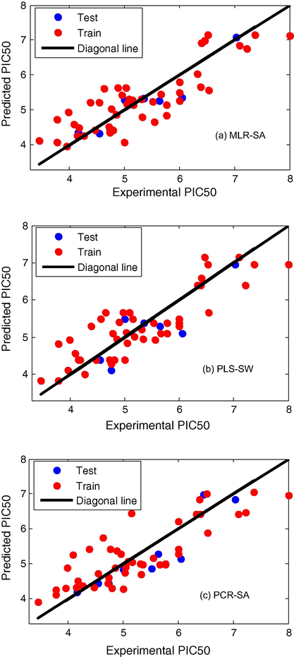
- Predicted (blue) versus experimental values (red) of biological activity: (a) MLR–SA, (b) PLS–SW, and (c) PCR–SA.

- Residual plot between predicted and experimental values: (a) MLR–SA, (b) PLS–SW, and (c) PCR–SA.
Although descriptors have an important role in identifying relationship with the activity, the exact interpretation of the conventional QSAR models has always been a challenging task. These models do not clearly specify the site at which modification is required in the molecules. For this purpose, 3D-QSAR models such as CoMFA have played a vital role (Cramer et al., 1988). The 3D-QSAR descriptors are steric and electrostatic fields calculated at the grid points generated around aligned set of molecules. As the descriptor pool is very large, 3D-QSAR models are generated by using regression methods such as Partial Least Squares (PLS) method, which can reduce the dimensionality. The 3D-QSAR models can provide clues for designing new molecules by specifying areas along with its steric and electrostatic requirements of the molecules. However, 3D-QSAR method has some limitation. Two of the major limitations of this method are its dependency on molecular alignment and conformers chosen for the alignment. This aspect becomes vital when there is not any information about bio-active conformation or when the molecular framework is not rigid. Recently Fragment based QSAR (Group based QSAR (G-QSAR)) has been developed which provides a method for better understanding of the structure activity relationship both in terms of identifying important chemical modifications at specific substitution sites and also by providing a mathematical model for the prediction of the activities of the new molecules. The site specific clues along with the interpretation of descriptors provided by G-QSAR will help medicinal chemists to design better molecules (Ajmani et al., 2009).
4 Conclusion
In conclusion, some novel sulfonamide derivatives as PCP inhibitors were studied by QSAR. The developed models reveal some useful structural information associated with inhibitory concentration. Sphere exclusion method was used to classify data into categories of train and test set. The generated models were analyzed and validated for their statistical significance, internal and external prediction power. QSAR study reveals descriptors which play important role in the biological activities of PCP inhibitors. Alignment Independent (AI) and Atomic valence connectivity index (chiv) are subclasses of physicochemical descriptors that have the greatest effect. The derived models can be useful in designing and synthesis of some new PCP inhibitors that can be used for treatment of fibrotic conditions.
Acknowledgments
The authors gratefully acknowledge partial support of this work by the Research Affairs Office of Bu-Ali Sina University (Grant number 32-1716 entitled as development of chemical methods, reagents and molecules).
References
- QSAR Comb. Sci.. 2009;28:36-51.
- Bioorg. Med. Chem. Lett.. 2008;18:6562-6567.
- Cardiovasc. Pathol.. 2010;19:191-192.
- Respir. Med.. 2014;108:224-226.
- J. Am. Chem. Soc.. 1988;110:5959-5967.
- Bioorg. Med. Chem. Lett.. 2002;12:1233-1235.
- Bioorg. Med. Chem. Lett.. 2000;10:2513-2516.
- Regression and Linear Models. New York: McGraw-Hill; 1990.
- Bioorg. Med. Chem. Lett.. 2003;13:2101-2104.
- J. Biol. Chem.. 2002;277:4223-4231.
- Toxicol. Appl. Pharmacol.. 2012;262:301-309.
- Statistics. Philadelphia, PA: W.B. Saunders Co.; 1976.
- J. Mol. Graphics Modell.. 2002;20:269-276.
- J. Chem. Inf. Comput. Sci.. 2003;43:144-154.
- J. Mach. Learn. Res.. 2003;3:1157-1182.
- Chem. Rev.. 2001;101:619-672.
- Cytokine Growth Factor Rev.. 2013;24:133-145.
- J. Biol. Chem.. 1985;260:15996-16003.
- Quant. Struct.-Act. Relat.. 1996;15:285-289.
- Ann. Thorac. Surg.. 1992;54:1053-1058.
- J. Chem. Phys.. 1953;21:1087-1092.
- Molecular Design Suite 3.5, VLife Technologies, Pune, India. (www.vlifesciences.com).
- Bioorg. Med. Chem. Lett.. 2003;13:2381-2384.
- J. Am. Acad. Dermatol.. 2002;46:S63-S97.
- J. Med. Chem.. 2003;46:3013-3020.
- Comput. Stat. Data Anal.. 2005;48:159-205.
- Bioorg. Med. Chem. Lett.. 2012;22:7397-7401.
- J. Mol. Cell Cardiol.. 2014;67:112-125.
- Nat. Rev. Immunol.. 2004;4:583-594.
- J. Chem. Inf. Model.. 1999;40:185-194.


