

Translate this page into:
Structure-odor relationship in pyrazines and derivatives: A physicochemical study using 3D-QSPR, HQSPR, Monte Carlo, molecular docking, ADME-Tox and molecular dynamics
⁎Corresponding author. t.lakhlifi@umi.ac.ma (Tahar LAKHLIFI)
-
Received: ,
Accepted: ,
This article was originally published by Elsevier and was migrated to Scientific Scholar after the change of Publisher.
Peer review under responsibility of King Saud University.
Abstract
In this study, using both 2D-QSPR and 3D-QSPR approaches, to understand the structure-odor relationship of 78 1–4-pyrazine odorant molecules and to use this knowledge for the design of new food and flavor products. According to our results, the developed models have good predictability such as the HQSPR/BC model with , = 0.916, CoMSIA/SEH model with = 0.624, = 0.590, = 0.932, = 0.963, and Topomer CoMFA model with = 0.899, = 0.916. The Monte Carlo method was used in the creation of a Quantitative Structure-Property Relationship (QSPR) model. The molecular structure is represented using optimized Simplified Molecular Input Line Entry System (SMILES) and molecular descriptors. The performance of the model is evaluated using the Correlation Ideality Index (IIC) and the Correlation Contradiction Index (CCI). The best model, designated as TF2, boasts excellent statistical properties with a training R-squared value of 0.957 and a test R-squared value of 0.834. The model was then used to determine promoter activity levels, which formed the basis for the design of 36 new odorant molecules. Molecular docking and pharmacokinetic properties were used to explain the mode of binding between the proposed compounds and the active site of the Porcine Odorant Binding Protein complexed with pyrazine (2-isobutyl-3-methoxypyrazine). Molecular dynamic simulation was used to assess and justify the stability of the ligand in the active site of the receptor. The results of this study provide a basis for the discovery of new compounds with lower olfactory thresholds and diverse pharmacological properties.
Keywords
Pyrazine
Odor
Monte-Carlo
Molecular Docking
MD simulation
3D/2D-QSAR

1 Introduction
The presence of volatile substances in perfumes, medicines and food chemistry is of particular importance for future industrial manufacturing. Volatile substances can accumulate either in the product itself or in the materials, producing undesirable odors that reduce the quality of the product. This is of great importance when the released volatiles have a strong odor, such as pyrazine derivatives, which are of great interest due to their high odor and flavor characteristics (Valdés García et al., 2021).
Pyrazine derivatives are heterocyclic nitrogen-containing compounds, which can be formed chemically by the condensation of two α-aminocarbonyl molecules such as amino acids or amino sugars. The two aminocarbonyl compounds first react to form a 1,4-dihydropyrazine and then undergo aromatization by oxidation in air or removal of a hydroxyl group to form the side chain, and can be extracted and distilled in small amounts directly from natural sources such as vegetables, coffee and cocoa or metabolically by various reaction processes (Mortzfeld et al., 2020) and (Ong et al., 2017).
Mechanism 1:
From alpha nitroso / nitro / azide Ketones by chemo-selective reduction (Zn/CH3CO2H) followed by spontaneous dimerization and subsequent oxidation leads to formation of pyrazine derivatives.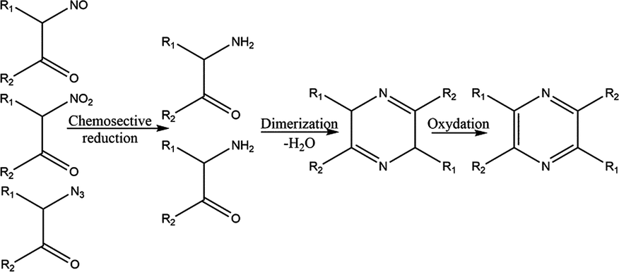
Mechanism 2:
From condensation reaction of alpha diketone whit 1,2-diaminoalkanes followed by oxidation in presence of CuCrO4 at 300 ⁰C leads to formation of pyrazine derivatives.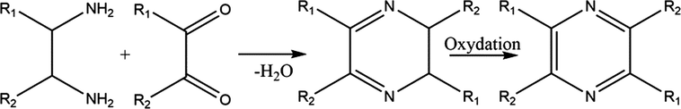
Mechanism 3:
Intermolecular diamino cyclization of ethylenediamine followed by dehydrogenation over copper chromite catalyst gives pyrazine.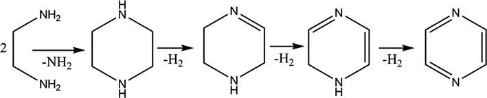
Mechanism 4:
From epoxide ring opening reaction with ethylenediamine followed by oxidation leads to formation of pyrazine derivatives.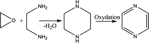
Mechanism 5:
Pyrazine is a six membered heterocyclic compound of the Diazines type derived from benzene by replacement of two –CH group by two nitrogen atoms at 1st and 4th position.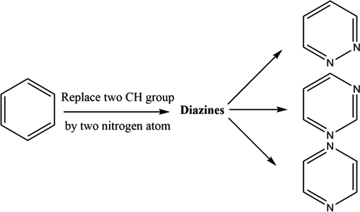
The experiment is a direct way of obtaining data on the activity and properties of molecules, but it has many disadvantages, such as the need for a myriad of test organisms, high cost, long time lag, the difference between values measured by different researchers, etc.
Therefore, it would be impossible to know the chemical and biological properties of all organic compounds by experiment. But with the rapid development of the theoretical study of computational chemistry and computer methods, it is possible to obtain the chemical properties of molecules quickly and accurately by molecular modeling. The quantitative structure–property relationship QSPR allows the interpretation and prediction of the property of new molecules (Ma, 2022).
3D-QSPR is one of the most widely used computational methods to predict molecular properties. This method has achieved remarkable success through constant progress in various fields such as medical, medicine, the pharmaceutical industry, and life sciences such as medicinal chemistry, materials science, and toxicology.
Numerous studies on the structure–property-activity relationship of pyrazine derivatives suggest that variations in odor activities depend on the type of substituent groups and the location of the attached substituents in the pyrazine ring, these studies also showed that there is a good relationship between the odor thresholds of di-substituted pyrazines that have hazelnut or brown notes, and proposed parameters elucidated from the retention indices for the respective substituent group (Belhassan et al., 2019).
Olfactory threshold studies of many alkylated pyrazine derivatives show that substituents located at the 2, 3, and 5 positions of the pyrazine ring should play an important role in odorant activity. Thus, flavor quality classification can be achieved with QSAR/QSPR studies through good predictive accuracy, integrated descriptor selection, and a method of evaluating the importance of each descriptor in the model (Chtita et al., 2018).
The QSPR approach encompasses many methods that correlate the property of molecules with physicochemical and/or structural properties. In this work, we developed two-dimensional models such as Hologram QSPR and Monte Carlo, and three-dimensional models such as Topomer CoMFA and CoMSIA for a series of 78 odorant molecules, we combined these four methods to generate the best models that collect and interpret complex data from a range of bioactive molecules to build computational models that correlate chemical properties and/or biological activity.
Through these approaches, the molecular features responsible for the odor threshold property of the studied compounds were identified using the best Topomer CoMFA and CoMSIA models. The Topomer CoMFA and CoMSIA models generate different contour maps which were then used to identify favored and unfavored regions in order to identify sites for enhancing the odorant property of the studied molecules. The HQSAR analysis suggested fragments with positive and negative contributions, which allowed the identification of fragments that gave insight into the main fragments responsible for increasing or decreasing the olfactory threshold, subsequently we are in the process of explaining the reliable predictive relationship of pyrazine odorant molecules using the CORAL software based on the Monte Carlo algorithm that has been widely used for QSPR model design. which applies the SMILES code to the molecules to calculate the correlation weight descriptor (CWD). This process is applied by different research groups for a large number of different medicinal, biochemical and physicochemical parameters. Predictability is the most important criterion for the QSPR model development process. To determine this criterion, many statistical methods have been reported in the literature. However, none of them is able to estimate the predictability of the QSPR model individually and all of them are related to each other. A new predictability parameter, the correlation ideality index (CII), has recently been suggested, which is based on the correlation coefficient and the mean absolute error. In 2019, the same authors introduced a new prediction parameter, namely the correlation contradiction index (CCI). It has been shown that there is a good correlation between the validation correlation coefficient and the CCI. In this work, the comparison of CCI and CCI was performed to select the best model, and thus to study the additional effect of CCI on CCI (Tabti et al., 2022b).
In addition, the statistical consistency of these developed models was assessed based on their correlation ability for the training set, as well as their predictive power for an external test set. We, therefore, propose quantitative models and attempt to interpret the properties of the compounds based on 2D-QSPR and 3D-QSPR analyses.
2 Materials and methods
2.1 Selection of the data set
In this new study, a series of 78 selected pyrazine derivatives with odor threshold (t) values were extracted from reference, these molecules were studied to build the CoMSIA, HQSPR, Topomer CoMFA, and monte Carlo models, 59 molecules were selected to propose the quantitative model (training set), and 19 molecules were used to test the performance and quality of the proposed model (test set). Table 1 shows the chemical structures of the studied molecules, and the property values of the experimental odor thresholds in log(1/t) (Belhassan et al., 2019). Odor threshold (t); Test set (*).
N°
R1
R2
R3
R4
Log(1/t)
N°
R1
R2
R3
R4
Log(1/t)
M1
H
H
H
H
3.523
M40
C5H11
SC2H5
H
H
9.000
M2
CH3
H
H
H
4.523
M41
C8H17
SC2H5
H
H
8.699
M3
C2H5
H
H
H
5.398
M42
C10H21
SC2H5
H
H
6.921
M4
C3H7
H
H
H
6.523
M43
H
SC6H5
H
H
6.398
M5
C4H9
H
H
H
6.398
M44
CH3
SC6H5
H
H
6.523
M6
C5H11
H
H
H
8.301
M45
C3H7
SC6H5
H
H
7.046
M7*
C6H13
H
H
H
6.699
M46
C5H11
SC6H5
H
H
8.000
M8
C7H15
H
H
H
7.000
M47
C8H17
SC6H5
H
H
7.097
M9*
C8H17
H
H
H
6.398
M48*
C10H21
SC6H5
H
H
6.523
M10*
C10H21
H
H
H
5.955
M49
H
OCH3
H
H
6.398
M11
CH3
H
H
CH3
6.398
M50*
CH3
OCH3
H
H
8.155
M12*
CH3
H
H
OCH3
7.770
M51
C2H5
OCH3
H
H
8.000
M13*
CH3
H
H
OC2H5
8.301
M52*
C3H7
OCH3
H
H
9.921
M14
CH3
H
H
SCH3
7.699
M53
C4H9
OCH3
H
H
10.301
M15
CH3
H
H
COCH3
6.523
M54*
C5H11
OCH3
H
H
10.699
M16
C2H5
H
H
CH3
7.398
M55*
C6H13
OCH3
H
H
10.155
M17
CH3
H
CH3
H
7.097
M56*
C7H15
OCH3
H
H
10.585
M18
CH3
H
OCH3
H
7.699
M57
C8H17
OCH3
H
H
10.222
M19*
CH3
H
OC2H5
H
7.921
M58
C10H21
OCH3
H
H
7.398
M20
CH3
H
SCH3
H
7.222
M59
(CH2)2CH(CH3)2
OCH3
H
H
11.201
M21*
CH3
H
COCH3
H
6.398
M60
(CH2)3CH = CH2
OCH3
H
H
10.523
M22
C2H5
H
CH3
H
7.796
M61
CH(CH3)C2H5
OCH3
H
H
10.398
M23*
CH3
CH3
H
H
6.097
M62
CH2CH(CH3)C3H7
OCH3
H
H
11.097
M24
C2H5
CH3
H
H
6.301
M63
CH2CH(CH3)2
OCH3
H
H
10.347
M25
C3H7
CH3
H
H
7.222
M64
CH2CH(CH3)C2H5
OCH3
H
H
10.921
M26*
CH(CH3)2
CH3
H
H
7.796
M65
(CH2)3CH(CH3)2
OCH3
H
H
11.222
M27
CH3
COCH3
H
H
7.699
M66
CH(CH3)2
OCH3
H
H
10.620
M28
H
SCH3
H
H
6.699
M67
(CH2)3CH = CHCH3 (E)
OCH3
H
H
9.886
M29*
CH3
SCH3
H
H
8.398
M68
(CH2)3CH = CHCH3 (Z)
OCH3
H
H
9.301
M30*
C2H5
SCH3
H
H
7.398
M69
H
OC2H5
H
H
7.097
M31
C3H7
SCH3
H
H
9.000
M70*
CH3
OC2H5
H
H
9.097
M32
C5H11
SCH3
H
H
9.921
M71
C2H5
OC2H5
H
H
7.699
M33
C8H17
SCH3
H
H
9.155
M72
C5H11
OC2H5
H
H
10.097
M34
C10H21
SCH3
H
H
7.699
M73
C8H17
OC2H5
H
H
8.699
M35
CH(CH3)2
SCH3
H
H
10.328
M74*
C10H21
OC2H5
H
H
7.222
M36
H
SC2H5
H
H
6.046
M75
H
OC6H5
H
H
7.523
M37
CH3
SC2H5
H
H
7.155
M76
CH3
OC6H5
H
H
6.699
M38
C2H5
SC2H5
H
H
7.222
M77
C5H11
OC6H5
H
H
7.301
M39
C4H9
SC2H5
H
H
8.398
M78
C10H21
OC6H5
H
H
7.155
2.2 Modelling and molecular alignment
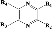
We used the Sybyl software to draw molecules from the database, and these registered molecules were reduced using molecular mechanics. We picked the Alignment database technique, which has a force field parameter (Tripos), an energy gradient convergence threshold of 0.01KCal/mol, and a charge type of Gasteiger-Hückel with a maximum of 1000 iterations. The structural alignment phase is included in the 3D-QSPR study because alignment is a necessary first step in statistical analyses of flexible structures in 3D-QSPR models (Vyas et al., 2017).
The alignment databases were chosen for their ability to produce satisfactory results, and the M65 compound was chosen as the model molecule against which the other compounds were matched (Fig. 1).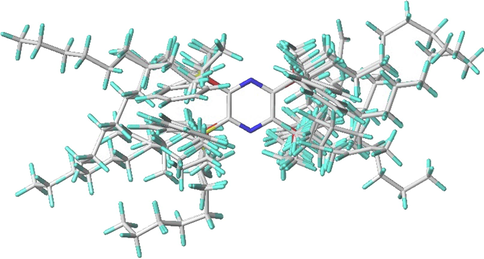
Database alignment.
2.3 Monte Carlo regression
The method for optimal hybrid descriptors is based on SMILES structures and molecular graphical representations, both of which are based on correlation weight optimization. The Monte Carlo regression model was created using the CORAL application (https://www.insilico.eu/Coral). CORAL works out as follows:
The molecular structure can be represented using SMILES and/or a molecular graph. The two molecular structure representations stated above have an effect on optimal hybrid descriptors. Maximizing the correlation weight of the SMILES attributes with the correlation weight of the chart invariants yields optimal hybrid descriptors. A parameter prediction model is fitted with the best DCW hybrid descriptor (T, N):
The optimum descriptor of the molecular feature function taken from SMILES is DCW (T, N). T and N are the best threshold and number of epochs determined during construction, respectively (Liman et al., 2022).
T is the threshold for classifying molecular qualities (structural features) into two groups: rare and frequent. If a structural feature is widespread in energizing substances, it can be linked to property; nevertheless, unusual features have less value and are viewed as noise. The weights of correlation (CW) of active structural attributes (ASs) are used to construct the ideal descriptor: for rare attributes, the CW is set to zero, signaling that they are not included in the model.
The N represents the number of times a DCW of a molecular characteristic is changed. The DCW values are obtained during construction using Monte Carlo optimization. The goal of the Monte Carlo approach is to maximize the correlation coefficient between the ideal descriptor and the parameter. Optimization is done with the formation and invisible formation ensembles to avoid over-formation (Toropov et al., 2020).
In this work, optimization was performed by balancing the correlations of the TF1 and TF2 target functions in the CORAL 2017 software to build the QSPR models, which are used to obtain the best results. In order to avoid over-training, the correlation balance method, which requires a high correlation between training and validation packages, was proposed.
2.4 Hologram-QSPR (HQSPR)
The Tripos HQSPR method is a computational approach for predicting molecular properties based on 2D molecular fragments. The method takes advantage of the fact that molecular properties can be correlated with the molecular structure, and that the molecular structure can be represented as a series of 2D molecular fragments.
In the first step of the HQSPR method, 2D molecular structures are divided into all possible linear and branched fragments, and each unique fragment is assigned a specific integer using a cyclic redundancy check (CRC) algorithm. These integers are then used to create a molecular hologram that serves as a structural descriptor, containing topological and compositional information about the molecular structure (Vyas et al., 2017).
In the second step, the molecular holograms are correlated with the corresponding biological properties using partial least squares (PLS) analysis. A drop-out cross-validation (LOOCV) is performed to identify the optimal number of explanatory variables or components that result in an optimal model. The final step involves deriving a mathematical regression equation that links the values or components of the molecular holograms with the corresponding biological properties.
The Tripos HQSPR method is a powerful tool for predicting molecular properties and has potential applications in fields such as drug discovery, materials science, and chemical engineering. By allowing for the automated analysis of large datasets, the Tripos HQSPR method can help speed up the process of discovering new drugs and materials, as well as improving our understanding of molecular structure–property relationships (Tabti et al., 2022c).
where
is the biological property of the ith compound, xij is the occupancy value of the molecular hologram of the ith compound at position or bin j, Cj is the coefficient for bin j derived from the PLS analysis, and L is the hologram length. One of the drawbacks of HQSPR is the fragment collision problem, which occurs during the fragment hashing process (Fig. 2).
Development of the predictive equation obtained by partial least squares analysis of the HQSPR model.
Although hashing reduces the length of the hologram, it results in different fragments in the same bin. The hologram length, a user-definable parameter, controls the number of bins in the hologram, and changing the hologram length can result in a change in the bin occupancy pattern. The program provides 12 default lengths but after several trials, we chose the first four which proved to give good predictive models on different data sets.
2.5 CoMFA and CoMSIA analysis
CoMSIA was created to address some of the shortcomings of CoMFA. In CoMSIA, molecular similarity indices derived from the modified SEAL similarity criteria are used as descriptors to account for steric, electrostatic, hydrophobic, and hydrogen bonding properties all at the same time. Individual indices are calculated by comparing the similarity of each molecule in the dataset to a common probe atom (with radius 1A, character + 1, and hydrophobicity + 1) located at the intersections of a surrounding grid/network. The mutual distance between the probe atom and the atoms in the aligned data set molecules is also considered when calculating similarity at all grid points (Wang et al., 2021).
Gaussian-like functions are used to characterize the distance dependence and calculate the molecular properties. Because the underlying Gaussian-like functional forms are “smooth” and free of singularities, their slopes are not as steep as those of the Coulomb and Lennard-Jones functions in CoMFA, thus eliminating the need for arbitrary cutoff limits. CoMSIA and CoMFA are included in the Sybyl software from Tripos Inc.
2.6 Topomer CoMFA
The CoMFA topomer method was developed to overcome the alignment issue in CoMFA; this technique takes into account not only the steric and electrostatic descriptors, but also the molecular topomer descriptors (Tabti et al., 2022a). A topomer is a molecular fragment with a single internal geometry or “Pose.” To produce better models, the two main fragmentation strategies (R1, R2, R3 and R4 – Common Core) were used (Fig 3). The calculation of steric and electrostatic fields is similar to the CoMFA approach.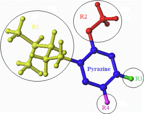
Cutting mode in Topomer CoMFA.
2.7 External validation plus
Validation is the most important stage in constructing quantitative structure–activity relationship (QSPR) models. It ensures the dependability of the final QSPR model as well as the acceptance of each phase in the model generation process. External validation (using an independent test set) is commonly employed to assess the predictive accuracy of a QSPR model (Ouabane et al., 2022).
The external predictivity of QSAR models is represented by computing and analyzing various validation metrics, which can be broadly classified into two classes or categories, namely, -based metrics such as , (F1), (F2), average , Δ , and purely error-based metrics such as root mean square error (RMSE), mean absolute error (MAE), and so on.
Furthermore, before doing external validation on a model, it is necessary to check for the presence of a systematic mistake that violates the basic assumptions of the least square’s regression model. If the model contains significant systematic error (bias), it should be ignored, and any external validation test performed on such a biased model is worthless.
External Validation Plus is a tool that checks for systematic errors in the model (only if the user chooses; optional) and then computes all of the required external validation parameters while evaluating the performance of a QSAR model's actual prediction quality using our recently proposed MAE-based criteria (Yu et al., 2023).
Systematic error is present when any one or more of the following conditions is true:
NPE: Number of positive errors, and NNE: Number of negative errors
MPE: Mean of positive error, MNE: Mean of negative errors, and ABS: Absolute value
AAE: Average of absolute prediction errors, and AE: Average of predictions errors
-
greater than 0.5 for residuals sorted on experimental response values
In the external Validation tool, the above threshold values are set as default and user can change the threshold values as required.
If any of the conditions listed above are met, the program will alert you to the presence of systematic error in the output file and recommend that you discard the model (only if the user chooses to check for systematic error). Furthermore, examining the external validity parameter is pointless if a systematic inaccuracy exists.
2.8 In silico pharmacokinetic ADME-Tox study
The ADME/Tox examination is a crucial step in the drug discovery process as it determines the pharmacokinetic properties of a drug candidate, including its absorption, distribution, metabolism, excretion, and toxicity. However, this process can be lengthy and costly, and not all drug candidates meet the required criteria (Ugale et al., 2017).
To overcome these limitations, there are now various online and offline tools available that can help predict ADME/Tox properties in silico. The online pkCSM tool and the SwissADMET online server are two examples of these tools. These tools use computer models and algorithms to estimate the pharmacokinetic properties of new compounds without the need for extensive experimental testing (Hajji et al., 2021a).
By using these online tools, researchers can quickly and cost-effectively predict the ADME/Tox properties of drug candidates, allowing them to make informed decisions about which candidates to pursue in the drug discovery process. This can contribute to speeding up the drug discovery process and increasing the success rate of developing new drugs.
2.9 Molecular docking study
The mechanism of action between olfactory receptors and odorant molecules is a crucial step in the development of new odorant molecules for use in various pharmaceutical, cosmetic and agro-food fields. In this study, molecular docking simulation is a useful tool to determine this binding between pyrazine derivatives and the active site of the protein responsible for the transmission of the odorant molecules and we have chosen a receptor (PDB ID: 1DZK) to make comparisons with the reference ligand 2-isobutyl-3-metoxypyrazine, this odorant molecule noted M63 in the data base (Fig. 4).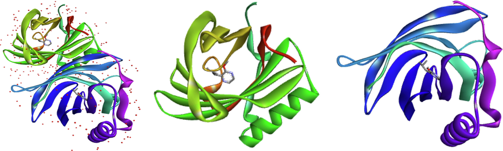
Representation of the crystalline structure 1DZK.pdb, chain A in green (ligand: 2-methoxy-3-(2-methylprop-2-en-1-yl) pyrazine) and chain B in blue (ligand: 2-methoxy-3-(2-methylpropyl) pyrazine).
In this study, we selected the most and least active compounds, which the reference ligand methoxypyrazine in the database on the one hand, and on the other hand the new compounds proposed from the molecule M65 with the highest odor threshold. All steps were performed by various available software such as CB-Dock (Ahfid et al., 2023), AM-Dock, Autodock-Vina (Mahfuz et al., 2022), Pyrex (En-nahli et al., 2022) and Sybyl. The molecular docking results were visualized by Discovery Studio (Hajji et al., 2021b).
The 3D structure of the receptor was chosen from the crystal structure (PDB ID: 1DZK) with a resolution of 1.48 Å, obtained from the RCSB protein database (https://www.rcsb.org). The structure of porcine odorant binding protein (pOBP) is a monomer of 157 amino acid residues, purified in abundance from porcine nasal mucosa. These residues were minimized by Sybyl software, then we added non-polar hydrogen atoms to the protein chain, Gasteiger-Huckel type charges were chosen, the convergence energy gradient was set to 0.01 kcal/mol maintaining 1000 times of optimization as the maximum limit cycle number.
The grid parameters are: positions P1: (x = 12.03, y = 4.71, z = 24.10), P2: (x = 14.65, y = 4.28, z = 25.12), dimensions (x = 30, y = 30, z = 30), energy range of order 10 and completeness equal to 8. We also used the re-Docking method to validate the Docking procedure, this technique based on the superposition of the M63 molecule after and the reference ligand were extracted before the molecular Docking, the RSMD value was displayed by the Discovery studio visualization software. Docking is reliable if the root means square deviation (RMSD) value is low (typically (1.5–2) Å depending on ligand size) (Shi et al., 2022).
2.10 Molecular dynamics simulations
To study the stability of complex (ligand–protein) interactions, molecular dynamic simulation (MD) calculations were performed on the best molecular docking poses. Using the CHARMM force field parameters, generate protein input files using the c solution generator and ligand topology using the CHARMM general force field Param-Chem server. The building blocks of the CHARMM-GUI solution consist of five steps. In the first step, the coordinates of the protein–ligand complex are read by the tool. The second step is to solve the protein–ligand complex and determine the shape and size of the system. and ions are added at this stage to neutralize the system. Periodic boundary conditions (PBC) are defined in the third step, which allows a large system to be approximated using a single cell which is then replicated in all directions. The simulation is only for atoms inside the PBC box. Bad contacts are removed at this stage by performing a short minimization. The fourth and fifth steps are to balance the system and production. Balancing is carried out in two steps: NVT and NPT, ensuring the system reaches the desired temperature and pressure (Koubi et al., 2023).
The input files for balancing and production are then downloaded and the desired changes are made, including the number of steps in the MD simulation, the frequency of trajectory recording and energy calculation, etc. GROMACS 2020.2 was used for both equilibration and production of all MD simulations. All complexes were first solvated in a cubic box of TIP3P water, then and ions were added to neutralize the net atomic charge of the whole system by randomly replacing the water molecules. Periodic boundary conditions (PBC) were imposed taking into account the shape and size of the system. The unrelated interactions were treated with a cut-off distance of 12 Å and the neighbors search list was buffered with the Verlet cut-off scheme, and the long-range electrostatic interactions were treated with the Ewald particle mesh method (SME) (Khaldan et al., 2022).
The CHARMM36 force field was applied to the protein–ligand complex. Prior to the production simulation, system energy minimization was performed using the gradient descent algorithm (5000 steps) (Balupuri et al., 2020). The complex was then balanced to stabilize its temperature and pressure by subjecting it to an NVT and NPT assembly and simulating it for 125 ps at a temperature of 300,15 K using 400 Kj. . and 40 Kj. . on the main axis and side chains respectively. Finally, the complex is subjected to a production simulation of 100 ns in NPT assembly at 300.15 K and 1 bar. To maintain the temperature, a Nose-Hoover thermostat was used and to maintain the pressure, a Parrinello-Rahman barostat was used. The LINCS algorithm was used to constrain hydrogen bonds using inputs provided by CHARMM-GUI. The 300 K V-rescale thermostat with a 1 ps coupling constant was used. The trajectories were recorded every 2 ps. Simulations of 100 ns in NPT assembly were performed for the production stage (Mahfuz et al., 2022).
2.10.1 Trajectory analysis
The GROMACS utilities have played a crucial role in the analysis of molecular dynamics (MD) simulations. Several specific tools have been used to study different aspects of protein–ligand complexes.
Firstly, the root mean square deviation (RMSD) was calculated to assess the stability of the complexes. This involved aligning the atoms of the main axis of the protein using the gmx_rms subroutine, which measures the similarity of atomic positions between the ligand and protein relative to a reference structure. Similarly, the root mean square fluctuations (RMSF) were calculated, focusing on the C-alpha atoms of the protein using gmx_rmsf. This analysis helped to identify regions of the protein with significant fluctuations (Mahmud et al., 2021).
The gyration radius of the protein atoms was also evaluated to assess the compactness and overall stability of the complex. This was done using the gmx_gyrate tool, which measures the spatial dispersion of protein atoms and provides an estimate of the gyration radius. In addition, hydrogen bond analysis was performed to evaluate specific interactions between the ligand and the protein. The gmx_hbond tool was used to calculate the number of hydrogen bonds formed within the protein–ligand interface. This provides information on the stability and nature of the interactions between the ligand and the protein. The distance between the center of mass of the protein and the ligand was measured during the simulation using the gmx_distance tool. This allows changes in the distance between the ligand and the protein to be tracked over time, providing insight into the dynamics of the binding (Alamri et al., 2020).
Finally, the molecular visualization program VMD was used to visualize the trajectories and analyze the frequency of protein–ligand contacts. VMD allows the visual observation of atomic movements during simulation, facilitating an intuitive understanding of molecular dynamics. Using VMD it is possible to analyze specific interactions between the protein and the ligand, examine atomic contacts and identify key residues involved in binding. The GROMACS utilities, such as gmx_rms, gmx_rmsf, gmx_gyrate, gmx_hbond and gmx_distance, complemented the analysis by providing quantitative measurements of the stability and structural properties of the protein–ligand complexes. This combination of tools allowed a comprehensive view of the molecular dynamics and associated interactions, providing an in-depth understanding of the stability of the studied complexes (El Bahi et al., 2023).
2.10.2 Binding free energy (MM/PBSA calculations)
For systems selected for further analysis, MM/PBSA (Molecular Mechanics/Surface Poisson-Boltzmann) calculations were performed using g_mmpbsa, a GROMACS tool used to calculate an estimated binding affinity. In general terms, the free energy of binding of the protein with the ligand solution can be expressed as follows:
Where is the total free energy of the protein–ligand complex, and are the total free energies of the isolated protein and the ligand in solution, respectively. g_mmpbsa can also be used to estimate the energy contribution per residue to the binding energy. To decompose the binding energy , and were first calculated separately for each residue and then summed to obtain the contribution of each residue to the binding energy. As g_mmpbsa only reads files from certain versions of GROMACS, the binary input file (.tpr) required for the MM-PBSA calculation with g_mmpbsa has been regenerated by GROMACS 5.1.4. The molecular structure file (.gro), the topology file (.top) and the MD parameter file (.mdp) were required to generate the binary input calculation file, and all came from the MD process (Wang et al., 2021).
3 Results and discussion
3.1 Results obtained by Monte-Carlo approach
QSPR model based on SMILES is a type of quantitative structure–property relationship model that uses Simplified Molecular Input Line Entry System (SMILES) notation to represent molecular structures. SMILES strings are used as input features to predict various physical and chemical properties of the molecules. The aim of such models is to establish a correlation between molecular structure and property, allowing for the prediction of properties for new molecules based on their SMILES representation. A total of 78 molecules were developed from two target function types, TF1 (without IIC) and TF2 (with IIC), using equations (TF1) and (TF2) respectively, to select consistent statistical performance.
The results of the statistical parameters obtained for the QSPR models generated from the odor threshold of odorant molecules based on SMILES descriptors for four sets randomly (+): Training set, (-): Invisible training, (#): Calibration and (*): test set are recorded in Table 2 and 3.
Model
data set
n
R2
CCC
IIC
Q2
s
MAE
F
TF1
Training set
20
0.7840
0.8789
0.5903
0.7435
0.868
0.719
65
Invisible training
20
0.7616
0.8442
0.5901
0.7067
0.897
0.632
57
Calibration
19
0.8173
0.8995
0.9003
0.7687
0.812
0.601
76
TF2
Training set
20
0.9569
0.9780
0.8004
0.9498
0.388
0.227
400
Invisible training
20
0.9721
0.9236
0.2833
0.9670
0.568
0.441
627
Calibration
19
0.9085
0.9422
0.7694
0.8830
0.577
0.441
169
ID
DCW
pt
Predpt
ID
DCW
pt
Predpt
TF1
TF2
TF1
TF2
TF1
TF2
TF1
TF2
1
+
55.770
67.320
3.523
4.160
3.536
36
–
72.748
86.036
6.046
5.436
6.125
3
+
74.751
79.918
5.398
5.587
5.279
37
–
98.735
91.093
7.155
7.390
6.824
4
+
74.000
89.805
6.523
5.530
6.646
42
–
107.482
91.797
6.921
8.048
6.922
11
+
81.913
89.392
6.398
6.125
6.589
49
–
89.558
87.033
6.398
6.700
6.263
24
+
100.243
87.544
6.301
7.503
6.333
57
–
118.463
107.293
10.222
8.873
9.065
32
+
109.747
112.572
9.921
8.218
9.795
60
–
128.819
112.482
10.523
9.652
9.782
35
+
123.836
114.872
10.328
9.277
10.113
64
–
139.419
114.324
10.921
10.449
10.037
38
+
110.494
93.982
7.222
8.274
7.224
66
–
138.902
112.926
10.620
10.410
9.844
40
+
111.505
105.874
9.000
8.350
8.869
67
–
126.771
107.886
9.886
9.498
9.147
43
+
86.209
88.167
6.398
6.448
6.419
73
–
120.220
101.236
8.699
9.005
8.227
45
+
96.890
91.885
7.046
7.251
6.934
2
#
66.562
83.485
4.523
4.971
5.772
46
+
96.344
99.818
8.000
7.210
8.031
8
#
74.150
88.928
7.000
5.542
6.525
51
+
117.679
100.234
8.000
8.814
8.088
14
#
82.222
95.491
7.699
6.149
7.432
53
+
121.497
112.478
10.301
9.101
9.782
17
#
94.710
87.950
7.097
7.087
6.389
58
+
116.854
101.662
7.398
8.752
8.286
20
#
87.157
98.742
7.222
6.520
7.882
59
+
151.407
122.185
11.201
11.350
11.124
31
#
110.293
104.639
9.000
8.259
8.698
68
+
126.771
109.021
9.301
9.498
9.304
34
#
105.725
98.495
7.699
7.916
7.848
69
+
87.815
92.783
7.097
6.569
7.058
39
#
112.126
102.613
8.398
8.397
8.417
77
+
107.473
100.862
7.301
8.047
8.175
41
#
109.091
97.428
8.699
8.169
7.700
78
+
103.450
86.785
7.155
7.745
6.228
44
#
89.263
89.049
6.523
6.678
6.542
5
–
76.379
91.297
6.398
5.709
6.852
47
#
93.931
91.372
7.097
7.029
6.863
6
–
75.759
94.559
8.301
5.663
7.304
61
#
138.725
118.240
10.398
10.397
10.579
15
–
82.153
88.669
6.523
6.143
6.489
62
#
138.484
119.332
11.097
10.379
10.730
16
–
93.540
92.755
7.398
7.000
7.054
63
#
147.345
112.683
10.347
11.045
9.810
18
–
102.224
95.174
7.699
7.652
7.389
65
#
151.783
121.308
11.222
11.379
11.003
22
–
104.032
95.690
7.796
7.788
7.460
71
#
125.561
95.111
7.699
9.407
7.380
25
–
101.231
93.559
7.222
7.578
7.165
72
#
122.634
109.683
10.097
9.187
9.395
27
–
102.717
94.668
7.699
7.690
7.319
75
#
93.399
89.146
7.523
6.989
6.555
28
–
74.491
90.601
6.699
5.567
6.756
76
#
100.391
90.093
6.699
7.515
6.686
33
–
107.334
104.126
9.155
8.037
8.627
The results indicate that the (TF2) model gives better results than the (TF1) model, which means that the addition of IIC (TF2) to the model weight improves its prediction. The comparison of experimental log(1/t) values to the calculated values for both models, presented in Table 4, clearly shows the statistical reliability of the TF2 models and that they meet the criteria established by external validation.
Test set
ID
DCW
Exp
TF1
TF2
Applicability
TF1
TF2
TF1
TF2
*
7
74.954
91.744
6.699
5.602
6.914
YES
YES
*
9
73.345
86.113
6.398
5.481
6.135
YES
YES
*
10
71.736
80.482
5.955
5.360
5.357
YES
YES
*
12
97.288
91.923
7.770
7.281
6.939
YES
YES
*
13
96.291
97.745
8.301
7.206
7.744
YES
YES
*
19
100.481
100.924
7.921
7.521
8.184
YES
YES
*
21
87.467
86.730
6.398
6.543
6.221
YES
YES
*
23
92.859
87.990
6.097
6.948
6.395
YES
YES
*
26
111.706
101.137
7.796
8.365
8.213
YES
YES
*
29
99.733
97.349
8.398
7.465
7.689
YES
YES
*
30
106.550
97.067
7.398
7.978
7.650
YES
YES
*
48
92.322
85.741
6.523
6.908
6.084
No
YES
*
50
114.799
95.403
8.155
8.598
7.420
YES
YES
*
52
121.422
107.806
9.921
9.096
9.136
YES
YES
*
54
120.876
115.740
10.699
9.055
10.233
YES
YES
*
55
120.072
112.924
10.155
8.994
9.844
YES
YES
*
56
119.267
110.109
10.585
8.934
9.454
YES
YES
*
70
113.802
92.222
9.097
8.523
8.980
YES
YES
*
74
118.611
95.606
7.222
8.884
7.448
YES
YES
3.1.1 Y-randomization test
Y-randomization is a tool used in the validation of QSPR/QSAR models that compares the performance of the original model in the data description (
) to models produced for permuted (randomly mixed) response, depending on the original model's descriptor directory and creation procedure. The validation method's results are presented in Table 5.
Training
Invisible training
Calibration
TF2
TF1
TF2
TF1
TF2
TF1
N
20
20
20
20
19
19
Origin
0.9569
0.7840
0.9721
0.7616
0.9085
0.8173
1
0.0086
0.0357
0.0016
0.3507
0.0681
0.0001
2
0.1002
0.0310
0.0070
0.0022
0.1032
0.1039
3
0.0279
0.0165
0.1187
0.0321
0.1032
0.1378
4
0.1570
0.1145
0.0128
0.0912
0.0022
0.0268
5
0.0805
0.0456
0.2302
0.0036
0.0528
0.0088
6
0.0184
0.0282
0.0022
0.0003
0.0356
0.1381
7
0.0035
0.0035
0.0766
0.1430
0.0147
0.0125
8
0.0180
0.0293
0.0000
0.0006
0.0926
0.0005
9
0.0355
0.0222
0.0203
0.0011
0.3408
0.0622
10
0.1139
0.0027
0.0024
0.1460
0.0251
0.0145
0.0563
0.0329
0.0472
0.0771
0.0940
0.0505
CRp2
0.9283
0.7674
0.9482
0.7220
0.8602
0.7916
The T threshold and N epochs were selected to produce the best statistical indicators for the calibration set. TF1 eliminates the effect of CII on the log (1/t) odor threshold and its predicted values differ from the experimental values, whereas in the case of TF2, which takes into account the influence of IIC on the odor threshold, the experimental odor threshold values are closer to the calculated values (Fig. 5). The (T, Nepoch) values for both TF1 and TF2 models demonstrate that the threshold and number of epochs are not identical.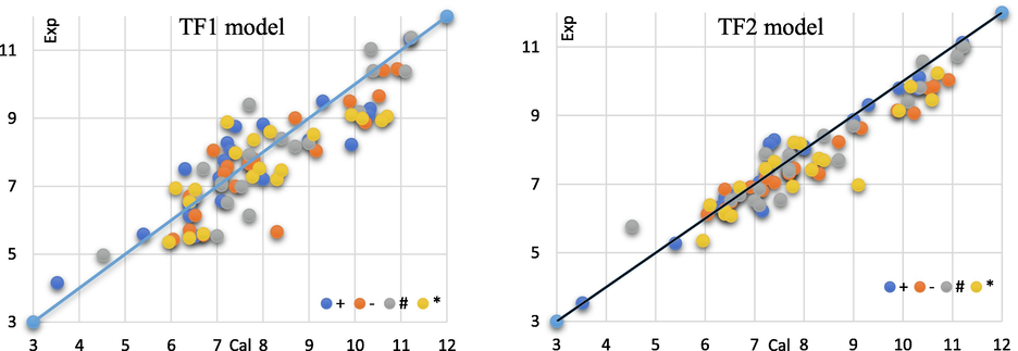
Models TF1 and TF2 were used to calculate the olfactory correlation thresholds of experimental odorous compounds.
3.1.2 Golbraikh and Tropsha’s criteria
The Golbraikh and Tropsha criteria are statistical parameters represented in the Table 6 below for evaluating the effectiveness of QSPR or QSAR models in computational chemistry. The criteria consist of two acceptance measures:
greater than 0.6 and
greater than 0.5(Elbouhi et al., 2022). These measures are commonly used to evaluate the accuracy of a predictive model in reproducing experimental data.
criteria
expression
Test set (TF2)
Test set (TF1)
interval
(1)
0.8336
0.6456
should be larger 0.5
(2)
0.8333
0.6425
should be larger 0.5
(3)
0.8088
0.5205
should be larger 0.5
0.0004
0.0048
should be lower 0.1
0.0298
0.1938
should be lower 0.1
K
K =
1.0511
1.0449
0.85 < k < 1.15
K’
K’ =
0.9461
0.9456
0.85 < k’ < 1.15
0.7023
0.4172
should be larger 0.5
0.8183
0.6098
should be larger 0.5
Average
Average
=
0.7603
0.5135
should be larger 0.5
Δ
Δ
0.1160
0.1925
should be lower 0.2
IIC
IIC=
0.3626
0.561
Low value
RMSE
0.7408
0.9766
Low value
MAE
MAE=
0.5680
0.8429
Low value
0.8052
0.5577
should be larger 0.5
3.2 Hologram-QSPR (HQSPR)
HQSPR is a new QSPR technique that avoids many problems associated with conventional 3D-QSPR approaches. Only structures and properties are required as input, no complex process of descriptor selection or 3D molecular alignment is required. HQSPR converts molecules in a data set into numbers of their constituent fragments. The fragment counting patterns from the molecules in the dataset is then linked to the targeted biological activity data using the PLS partial least squares analysis. Both steps, fragment counting, and PLS analysis are very fast. Nevertheless, the method is robust and highly predictive for many data sets. holograms 53, 59, 61, and 71 were chosen with a fragment number varying between 4 and 7 to construct all possible combinations of the Atoms, Bonds, Connections, Hydrogen Atoms, Chirality, and number of donor/acceptor hydrogens that are represented in Table 7.
Model
Fragment distinction
Component
SEE
SEE
Best Length
1
A
5
0.759
0.887
0.870
0.651
71
2
B
5
0.779
0.849
0.863
0.670
61
3
C
6
0.823
0.768
0.905
0.562
61
4
H
5
0.511
1.265
0.568
1.057
53
5
Ch
5
0.512
1.266
0.569
1.058
54
6
DA
5
0.720
0.957
0.856
0.686
71
7
A/B
5
0.702
0.987
0.816
0.776
71
8
A/C
5
0.724
0.950
0.861
0.674
61
9
A/H
6
0.734
0.941
0.870
0.659
71
10
A/Ch
5
0.746
0.912
0.857
0.685
71
11
A/DA
6
0.709
0.985
0.867
0.667
61
12
B/C
6
0.832
0.748
0.916
0.528
59
13
B/H
5
0.779
0.849
0.863
0.670
61
14
B/Ch
5
0.779
0.849
0.863
0.670
61
15
B/DA
6
0.673
1.044
0.868
0.663
71
16
C/H
6
0.823
0.768
0.905
0.562
61
17
C/Ch
6
0.823
0.768
0.905
0.562
61
18
C/DA
5
0.723
0.951
0.849
0.703
53
19
H/Ch
5
0.511
1.265
0.658
1.057
53
20
H/DA
5
0.720
0.957
0.856
0.686
71
21
Ch/DA
6
0.710
0.983
0.858
0.687
71
22
A/B/C
6
0.740
0.930
0.892
0.600
61
23
A/B/H
6
0.713
0.977
0.862
0.677
61
24
A/B/Ch
5
0.716
0.964
0.834
0.736
71
25
A/B/DA
6
0.712
0.98
0.864
0.674
71
26
A/C/H
6
0.766
0.883
0.886
0.616
71
27
A/C/Ch
5
0.724
0.951
0.861
0.673
61
28
A/C/DA
6
0.726
0.956
0.882
0.628
53
29
A/H/Ch
4
0.710
0.965
0.823
0.754
53
29
B/Ch/DA
6
0.676
1.039
0.864
0.673
71
30
A/H/DA
6
0.721
0.964
0.870
0.659
59
31
A/Ch/DA
4
0.703
0.977
0.811
0.780
59
32
B/C/H
6
0.832
0.748
0.916
0.528
59
33
B/C/Ch
6
0.832
0.748
0.916
0.528
59
34
B/C/DA
6
0.746
0.920
0.88
0.633
53
35
B/H/Ch
5
0.779
0.849
0.863
0.670
61
36
B/H/DA
6
0.673
1.044
0.868
0.633
71
37
C/H/Ch
6
0.823
0.768
0.905
0.562
61
38
C/H/DA
5
0.723
0.951
0.849
0.703
53
40
C/Ch/DA
6
0.710
0.983
0.858
0.687
71
41
H/Ch/DA
6
0.817
0.781
0.903
0.568
59
42
A/B/C/H
6
0.739
0.933
0.891
0.603
61
43
A/B/C/Ch
6
0.732
0.945
0.886
0.617
53
44
A/B/C/DA
6
0.736
0.937
0.866
0.667
61
45
A/B/H/Ch
5
0.748
0.907
0.873
0.645
61
46
A/B/H/DA
5
0.757
0.892
0.870
0.653
71
47
A/C/H/Ch
5
0.753
0.898
0.874
0.642
71
48
A/C/H/DA
6
0.832
0.748
0.916
0.528
59
49
B/C/H/Ch
6
0.746
0.920
0.880
0.633
53
50
B/C/H/DA
6
0.719
0.968
0.858
0.688
53
51
C/H/Ch/DA
6
0.676
1.039
0.864
0.673
71
52
B/H/Ch/DA
6
0.676
0.955
0.882
0.627
53
53
B/C/Ch/DA
5
0.725
0.948
0.851
0.699
59
54
A/H/Ch/DA
6
0.747
0.919
0.887
0.615
53
55
A/C/Ch/DA
5
0.720
0.956
0.847
0.706
59
56
A/B/Ch/DA
6
0.726
0.955
0.882
0.627
53
57
A/B/C/H/Ch
6
0.794
0.829
0.897
0.586
59
58
A/B/C/H/DA
6
0.777
0.863
0.90
0.577
59
59
A/B/C/Ch/DA
5
0.704
0.984
0.857
0.685
53
60
A/B/H/Ch/DA
5
0.756
0.894
0.873
0.643
61
61
A/C/H/Ch/DA
6
0.758
0.899
0.893
0.596
59
62
B/C/H/Ch/DA
6
0.726
0.955
0.882
0.627
53
63
A/B/C/H/CH/DA
6
0.744
0.924
0.890
0.604
59
A total of 63 models obtained using HQSPR shows that the Bonds and Connection fragments are explanatory fragments (comparison between the following models: 12, 32, 33 and 63) which generated the olfactory threshold prediction on the other hand we find that no effect of Hydrogen fragments Atoms and Chirality as a result of many of the donor and acceptor hydrogens having a negative effect on the statistical values of the prediction of the targeted biological property at cause of absence of donor groups, asymmetric carbons, enantiomers, and diastereomers except that two conformations E (M67) and Z M(68) among the 78 odorant molecules. Model 12 (Bonds/Connections) was chosen to develop the number of atoms connecting for each fragment, the set of results obtained present in Table 8.
Model
Fragment distinction
Component
SEE
SEE
Best Length
1–4
B/C
6
0.746
0.92
0.828
0.758
71
B/C/H
6
0.746
0.92
0.828
0.758
71
B/C/H/Ch
6
0.746
0.92
0.828
0.758
71
2–5
B/C
6
0.792
0.832
0.867
0.667
53
B/C/H
6
0.792
0.832
0.867
0.667
53
B/C/H/Ch
6
0.792
0.832
0.867
0.667
53
3–6
B/C
6
0.812
0.791
0.895
0.590
61
B/C/H
6
0.812
0.791
0.895
0.590
61
B/C/H/Ch
6
0.812
0.791
0.895
0.590
61
4–7
B/C
6
0.832
0.748
0.916
0.528
59
B/C/H
6
0.832
0.748
0.916
0.528
59
B/C/H/Ch
6
0.832
0.748
0.916
0.528
59
5–8
B/C
6
0.826
0.762
0.906
0.560
53
B/C/H
6
0.826
0.762
0.906
0.560
53
B/C/H/Ch
6
0.826
0.762
0.906
0.560
53
6–9
B/C
6
0.798
0.820
0.913
0.539
61
B/C/H
6
0.798
0.820
0.913
0.539
61
B/C/H/Ch
6
0.798
0.820
0.913
0.539
61
7–10
B/C
5
0.735
0.932
0.856
0.685
53
B/C/H
5
0.735
0.932
0.856
0.685
53
B/C/H/Ch
5
0.735
0.932
0.856
0.685
53
8–11
B/C
5
0.738
0.925
0.831
0.744
59
B/C/H
5
0.738
0.925
0.831
0.744
59
B/C/H/Ch
5
0.738
0.925
0.831
0.744
59
9–12
B/C
6
0.708
0.987
0.827
0.760
71
B/C/H
6
0.708
0.987
0.827
0.760
71
B/C/H/Ch
6
0.708
0.987
0.827
0.760
71
10–13
B/C
5
0.710
0.974
0.802
0.805
71
B/C/H
5
0.710
0.974
0.802
0.805
71
B/C/H/Ch
5
0.710
0.974
0.802
0.805
71
11–14
B/C
6
0.604
1.149
0.723
0.962
61
B/C/H
6
0.604
1.149
0.723
0.962
61
B/C/H/Ch
6
0.604
1.149
0.723
0.962
61
The change in the number of fragment connections demonstrates what we previously stated; on the other hand, our choice of starting point, minimum and maximum number of atoms in a fragment yields good results, as shown in the picture below (Fig. 6).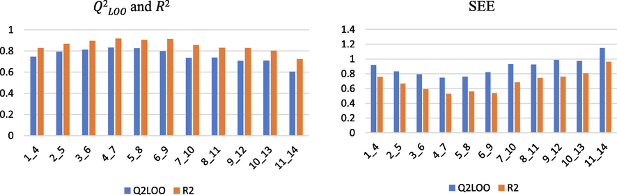
The influence of the minimum and maximum number of atoms has an impact on the model performance (B/C).
3.2.1 PLS HQSPR-Hologram
In this work, a PLS technique was used to compare the prediction values of each Hologram (53, 59, 61, 71, and AVG) and to establish the best fragment of the HQSPR predictive models represented in Table 9.
N
pt
59
71
61
53
AVG
N
pt
59
71
61
53
AVG
Training set
M1
3.52
3.76
4.81
4.60
4.39
4.39
M57
10.22
9.06
9.14
9.12
9.14
9.11
M2
4.52
5.17
5.39
5.12
5.49
5.29
M58
7.40
8.22
8.24
8.36
8.43
8.31
M3
5.40
5.59
5.84
5.83
5.57
5.71
M59
11.20
11.20
10.90
10.94
10.89
10.98
M4
6.52
6.06
6.26
6.49
6.08
6.22
M60
10.52
9.69
9.65
9.97
9.66
9.74
M5
6.40
7.16
7.05
6.99
6.59
6.95
M61
10.40
10.70
11.48
10.89
10.98
11.01
M6
8.30
7.46
7.39
7.31
7.00
7.29
M62
11.10
11.43
11.24
11.57
11.52
11.44
M8
7.00
6.77
6.68
6.73
6.22
6.60
M63
10.35
10.27
10.07
10.02
10.24
10.15
M11
6.40
7.00
5.68
6.03
6.19
6.23
M64
10.92
11.46
11.11
11.10
10.80
11.12
M14
7.70
8.24
7.54
8.14
7.87
7.95
M65
11.22
10.28
10.55
10.81
11.16
10.70
M15
6.52
6.41
7.44
7.18
6.98
7.00
M66
10.62
10.09
10.30
10.00
10.13
10.13
M16
7.40
6.62
7.04
7.15
7.51
7.08
M67
9.89
9.67
9.53
10.17
9.29
9.66
M17
7.10
7.28
6.67
6.31
6.85
6.78
M68
9.30
9.67
9.53
10.17
9.29
9.66
M18
7.70
7.55
7.60
7.59
7.67
7.60
M69
7.10
6.11
6.08
5.88
5.83
5.98
M20
7.22
7.55
7.60
7.59
7.67
7.60
M71
7.70
7.67
7.57
7.71
7.76
7.68
M22
7.80
7.66
7.85
7.57
7.90
7.74
M72
10.10
9.51
9.36
9.22
9.44
9.38
M24
6.30
6.45
6.40
6.22
6.99
6.51
M73
8.70
8.41
8.20
8.26
8.31
8.30
M25
7.22
6.79
6.79
6.84
7.26
6.92
M75
7.52
6.91
6.46
6.55
6.85
6.69
M27
7.70
8.01
7.86
7.97
7.50
7.83
M76
6.70
6.67
6.31
6.75
6.46
6.55
M28
6.70
6.54
6.76
6.76
6.57
6.66
M77
7.30
8.19
8.47
8.13
8.16
8.24
M31
9.00
8.93
9.19
9.09
9.42
9.16
M78
7.16
6.23
6.42
6.41
6.33
6.35
M32
9.92
10.17
10.30
10.07
10.26
10.20
Test set
M7
6.70
7.19
7.12
7.11
6.58
7.00
M33
9.16
9.06
9.14
9.12
9.14
9.11
M9
6.40
6.35
6.23
6.35
5.87
6.20
M34
7.70
8.22
8.24
8.36
8.43
8.31
M10
5.96
5.50
5.34
5.59
5.17
5.40
M35
10.33
10.09
10.30
10.00
10.13
10.13
M12
7.77
8.24
7.54
8.14
7.87
7.95
M36
6.05
6.11
6.08
5.88
5.83
5.98
M13
8.30
7.80
6.96
7.35
7.13
7.31
M37
7.16
7.15
7.04
6.78
6.98
6.99
M19
7.92
7.12
6.92
6.71
6.94
6.92
M38
7.22
7.67
7.57
7.71
7.76
7.68
M21
6.40
7.03
6.76
7.20
7.23
7.06
M39
8.40
9.22
9.02
8.90
9.04
9.04
M23
6.10
6.50
5.89
5.30
6.65
6.08
M40
9.00
9.51
9.36
9.22
9.44
9.38
M26
7.80
7.19
7.57
7.80
8.20
7.69
M41
8.70
8.41
8.20
8.26
8.31
8.30
M29
8.40
7.88
7.85
7.83
7.70
7.81
M42
6.92
7.56
7.31
7.50
7.61
7.49
M30
7.40
8.33
8.51
8.57
8.58
8.50
M43
6.40
6.91
6.46
6.55
6.85
6.69
M48
6.52
6.23
6.42
6.41
6.33
6.35
M44
6.52
6.67
6.31
6.75
6.46
6.55
M50
8.16
7.88
7.85
7.83
7.70
7.81
M45
7.05
6.94
7.36
7.15
7.31
7.19
M52
9.92
8.93
9.19
9.09
9.42
9.16
M46
8.00
8.19
8.47
8.13
8.16
8.24
M54
10.70
10.17
10.30
10.07
10.26
10.20
M47
7.09
7.08
7.31
7.17
7.03
7.15
M55
10.16
9.91
10.03
9.88
9.84
9.91
M49
6.40
6.54
6.76
6.76
6.57
6.66
M56
10.59
9.49
9.58
9.50
9.49
9.51
M51
8.00
8.33
8.51
8.57
8.58
8.50
M70
9.10
7.15
7.04
6.78
6.98
6.99
M53
10.30
9.88
9.95
9.75
9.86
9.86
M74
7.22
7.56
7.31
7.50
7.61
7.49
Following comparing the predicted values of each Hologram, we can see that Hologram 59 produces excellent results; we will apply this model to continue research investigation, and we will show the correlation between experimental and calculated values in the image below (Fig. 7).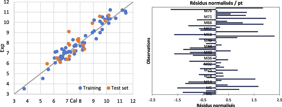
Residual graphs between experimental and predicted for HQSPR models.
3.2.2 HQSPR contribution map
The QSPR analysis focused on the contributions of biologically owned fragments of odorous molecules for each individual compound. The graphical results of the atomic contribution maps of the M65 compounds with the highest olfactory threshold value are represented in the color-coded structure diagram in Fig. 8.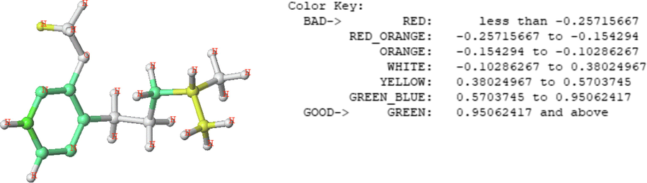
The HQSPR model contribution map on the M65 compound, and the coefficient of influence of each contribution.
The color of each atom implies its contribution to the olfactory threshold of the compound. The green color (green–blue, and yellow) represents a positive effect while the red color (red, red–orange, and orange) reflects the negative contribution to the olfactory threshold, and the intermediate contributions are white.
3.3 CoMSIA statistical results
Indicates Comparative Molecular Similarity Indices Analysis (CoMSIA), a statistical method used in molecular biology and computational chemistry to study the relationship between chemical structures and biological activity. The results summarized in Table 10 possibly reflect the results of different combinations of molecular descriptors used as inputs to the CoMSIA model, and their impact on the accuracy and robustness of the model. The goal of these tests is probably to determine the optimal combination of descriptors that provide the best prediction of biological activity for a given set of molecules.
CoMSIA Fields
N
SEE
F
S
E
H
A
D
S
0.582
0.581
0.880
0.917
6
0.632
63.517
1
–
–
–
–
E
0.551
0.551
0.698
0.769
7
1.013
16.858
–
1
–
–
–
H
0.539
0.527
0.965
0.980
9
0.354
148.025
–
–
1
–
–
D
–
–
–
–
–
–
–
–
–
–
–
–
A
0.061
0.064
0.023
0.038
1
1.724
1.330
–
–
–
–
1
S + E
0.619
0.655
0.900
0.971
6
0.557
78.023
0.661
0.339
–
–
–
S + H
0.543
0.560
0.958
0.971
8
0.381
142.757
0.379
–
0.621
–
–
S + A
0.642
0.662
0.903
0.924
6
0.569
80.566
0.917
–
–
0.083
–
E + H
0.598
0.579
0.917
0.957
6
0.527
95.392
–
0.294
0.706
–
–
E + A
0.465
0.525
0.792
0.848
6
0.833
32.931
–
0.938
–
0.062
–
H + A
0.485
0.482
0.937
0.960
7
0.440
120.331
–
–
0.958
0.042
–
S + E + H
0.289
0.318
0.532
0.545
1
1.193
64.765
0.282
0.268
0.450
–
–
0.473
0.525
0.683
0.741
2
0.990
60.830
0.287
0.277
0.436
–
–
0.573
0.573
0.800
0.854
3
0.795
73.153
0.294
0.272
0.434
–
–
0.596
0.613
0.860
0.900
4
0.671
82.827
0.299
0.256
0.445
–
–
0.609
0.617
0.909
0.944
5
0.546
105.636
0.303
0.236
0.461
–
–
0.624
0.590
0.932
0.963
6
0.476
118.784
0.305
0.228
0.467
–
–
0.624
0.594
0.946
0.968
7
0.427
128.379
0.305
0.219
0.475
–
–
0.624
0.655
0.962
0.978
8
0.361
160.209
0.305
0.206
0.489
–
–
0.624
0.636
0.972
0.984
9
0.312
191.975
0.303
0.196
0.502
–
–
0.624
0.603
0.979
0.990
10
0.275
224.979
0.303
0.190
0.507
–
–
0.624
0.559
0.984
0.991
11
0.243
261.715
0.301
0.185
0.515
–
–
0.624
0.539
0.986
0.992
12
0.228
274.464
0.302
0.181
0.518
–
–
0.624
0.633
0.989
0.996
13
0.214
287.891
0.303
0.179
0.518
–
–
0.624
0.627
0.990
0.994
14
0.199
310.288
0.304
0.175
0.520
–
–
0.624
0.602
0.990
0.995
15
0.196
298.812
0.305
0.176
0.519
–
–
0.624
0.571
0.991
0.997
16
0.189
301.692
0.304
0.175
0.521
–
–
S + E + A
0.636
0.608
0.888
0.927
5
0.605
84.129
0.578
0.335
–
0.087
–
S + H + A
0.573
0.570
0.957
0.976
8
0.387
138.348
0.380
–
0.571
0.048
–
E + H + A
0.613
0.604
0.899
0.927
5
0.576
93.9170
–
0.315
0.635
0.051
–
S + E + H + A
0.639
0.606
0.931
0.955
6
0.481
116.349
0.296
0.227
0.434
0.043
–
The combination of different 3D-CoMSIA fields with their results is a technique used to improve the performance and reliability of QSPR/QSAR models. This approach combines multiple molecular descriptors and multiple modeling algorithms to produce a more accurate and robust model. The search for this combination depends on the optimal number of components (N) choice, most of the later works use the standard Sybyl software parameters, but in our work, we studied the optimal number of component variation with respect to other statistical parameters to determine the relationship between them. The results obtained are represented in the Table 11.
Equation
Correlation
= 0.144*ln(N) + 0.650
R2 = 0.858
= 0.159*ln(N) + 0.600
R2 = 0.919
= 0.095*ln(N) + 0.405
R2 = 0.718
SEE = -0.390*ln(N) + 1.200
R2 = 0.988
F = 19.588*N + 17.653
R2 = 0.961
In this part, we determine the optimal number of components N of the 3D-QSPR model using the Comparative molecular similarity indices analysis (CoMSIA/SEH) method studied, we choose the parameters
,
,
,
, SEE and F to find the optimal number of components, It can be seen that the f-test value is proportional to the number of optimal components in a linear way, but the other parameters
,
,
and SEE are proportional to the number of optimal components in a logarithmic way, N = 6 maximum threshold of
, N = 10 maximum threshold of (
, and
) and N = 13 maximum threshold of SEE, according to the maximum value of
, we choose the optimal number of components N = 6 (Fig. 9).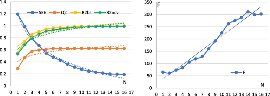
Graphical representation of each parameter studied as a function of the number of optimal components.
Upon determining the best number of components to be N = 6, it was found that the CoMSIA/SEH model can be trusted to give an explanation and prediction of the olfactory threshold of pyrazine derivative odor molecules. The results of the prediction and the comparison between the calculated and observed olfactory threshold are presented in Table 12 and Fig 10.
N
pt
S
E
H
Predpt
Residu
N
pt
S
E
H
Predpt
Residu
Training set
M1
3.52
2.28
0.44
0.81
3.89
−0.37
M57
10.22
4.90
0.46
3.52
9.20
1.02
M2
4.52
2.66
0.48
1.41
4.63
−0.11
M58
7.40
5.30
0.47
3.91
7.96
−0.56
M3
5.40
3.02
0.47
1.75
5.59
−0.19
M59
11.20
4.27
0.45
2.83
10.80
0.40
M4
6.52
3.34
0.47
2.08
6.34
0.18
M60
10.52
4.04
0.49
2.75
10.33
0.19
M5
6.40
3.66
0.47
2.42
6.91
−0.51
M61
10.40
4.06
0.44
2.46
10.49
−0.09
M6
8.30
3.96
0.47
2.75
7.37
0.93
M62
11.10
4.56
0.45
3.05
11.35
−0.26
M8
7.00
4.47
0.48
3.22
6.96
0.04
M63
10.35
4.05
0.44
2.54
10.78
−0.43
M11
6.40
2.99
0.52
1.86
6.29
0.11
M64
10.92
4.31
0.45
2.83
11.20
−0.28
M14
7.70
3.05
0.47
2.05
7.47
0.23
M65
11.22
4.57
0.43
3.10
10.97
0.25
M15
6.52
3.22
0.67
1.76
6.70
−0.18
M66
10.62
3.75
0.42
2.21
10.39
0.23
M16
7.40
2.87
1.55
2.36
7.35
0.05
M67
9.89
4.25
0.47
2.94
10.44
−0.56
M17
7.10
2.99
0.51
1.83
6.81
0.29
M68
9.30
4.27
0.49
2.88
9.79
−0.49
M18
7.70
3.06
0.47
1.42
7.52
0.18
M69
7.10
3.11
0.43
0.99
6.95
0.15
M20
7.22
3.06
0.44
2.01
7.94
−0.72
M71
7.70
3.73
0.50
2.13
7.86
−0.16
M22
7.80
3.20
1.55
2.58
7.81
−0.02
M72
10.10
4.56
0.48
2.97
9.37
0.73
M24
6.30
3.36
0.51
2.48
6.70
−0.40
M73
8.70
5.24
0.49
3.70
8.70
0.00
M25
7.22
3.66
0.51
2.74
7.43
−0.21
M75
7.52
3.57
0.41
2.65
7.30
0.23
M27
7.70
3.23
0.49
1.58
7.78
−0.08
M76
6.70
3.92
0.44
3.23
6.02
0.68
M28
6.70
2.74
0.43
1.59
6.71
−0.01
M77
7.30
4.93
0.43
4.13
7.75
−0.44
M31
9.00
3.69
0.44
2.89
8.51
0.49
M78
7.16
5.91
0.45
4.99
6.87
0.29
M32
9.92
4.28
0.45
3.50
9.54
0.38
Test set
M7
6.70
4.23
0.48
2.98
7.09
−0.40
M33
9.16
4.99
0.46
4.15
9.73
−0.57
M9
6.40
4.69
0.49
3.46
6.87
−0.47
M34
7.70
5.40
0.47
4.47
7.62
0.08
M10
5.96
5.11
0.49
3.84
6.82
−0.86
M35
10.33
3.74
0.45
2.80
9.29
1.04
M12
7.77
3.07
0.49
1.44
7.63
0.14
M36
6.05
3.05
0.41
1.76
6.92
−0.88
M13
8.30
3.41
0.47
1.61
8.63
−0.33
M37
7.16
3.37
0.45
2.52
6.80
0.36
M19
7.92
3.36
0.47
1.65
8.25
−0.33
M38
7.22
3.67
0.44
2.77
7.73
−0.51
M21
6.40
3.19
0.55
1.85
7.69
−1.29
M39
8.40
4.23
0.44
3.24
8.47
−0.07
M23
6.10
3.02
0.52
2.19
5.87
0.23
M40
9.00
4.49
0.44
3.48
8.80
0.20
M26
7.80
3.69
0.51
2.60
7.43
0.36
M41
8.70
5.13
0.45
4.06
8.12
0.58
M29
8.40
3.08
0.45
2.35
7.22
1.18
M42
6.92
5.52
0.46
4.40
7.26
−0.34
M30
7.40
3.41
0.45
2.64
7.76
−0.36
M43
6.40
3.56
0.42
3.07
5.75
0.65
M48
6.52
5.88
0.47
5.24
8.16
−1.64
M44
6.52
3.88
0.46
3.63
6.59
−0.07
M50
8.16
3.08
0.46
1.66
7.74
0.42
M45
7.05
4.37
0.44
4.03
7.78
−0.73
M52
9.92
3.70
0.45
2.28
9.73
0.19
M46
8.00
4.86
0.46
4.42
7.95
0.05
M54
10.70
4.22
0.45
2.82
10.30
0.40
M47
7.09
5.47
0.46
4.96
6.77
0.31
M55
10.16
4.46
0.45
3.07
10.05
0.10
M49
6.40
2.75
0.43
0.70
6.54
−0.14
M56
10.59
4.69
0.46
3.30
9.69
0.89
M51
8.00
3.41
0.45
1.98
9.02
−1.02
M70
9.10
3.43
0.48
1.83
7.98
1.12
M53
10.30
3.97
0.45
2.56
10.23
0.07
M74
7.22
5.65
0.49
4.10
8.66
−1.43
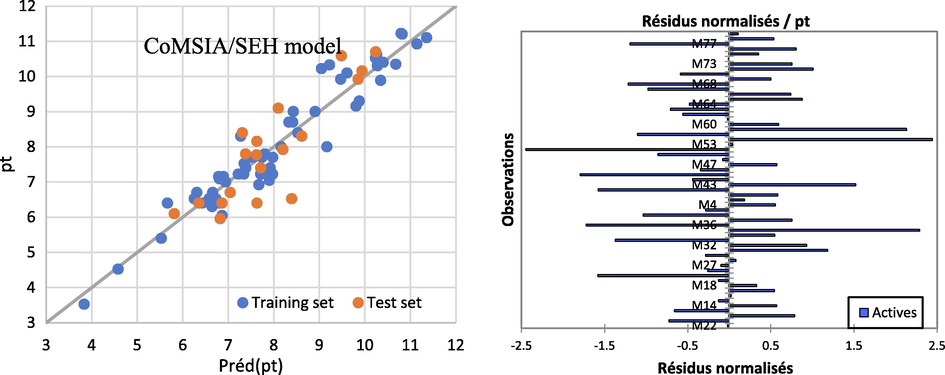
Graph of observed and calculated properties for training set and test set process based on the CoMSIA model.
3.3.1 CoMSIA contour map analysis
The molecule M65 was chosen to display the contribution of steric, electrostatic and hydrophobic fields represented in Fig 11: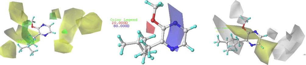
Contribution map of CoMSIA/SEH model on the compound M65.
- Steric: the steric congestion between the R1 ((CH2)3CH (CH3)2) and R2 (OCH3) substitutions of the M65 molecule promotes a steric field of 80% in green and 20% unfavorable in yellow shown in Fig. 11. The volume occupied by the methoxy group in space produces steric genes with branched substitutions more than linear substitutions, this explains that the olfactory threshold of compound M65 (log (1/t) = 11.222) smaller than M58 (log (1/t) = 7.398, R1 (C10H21), R2 (OCH3)), M54 (log (1/t) = 10.699, R1 (C5H11) and R2 (OCH3)). On the other hand, the favorable steric field clutter of hydrogen atoms in positions R3 and R4 is too small. This steric resistance is often used to propose new odor molecules.
- Electrostatic: a favorable electropositive field in blue color around the atoms of nitrogen of the common structure of pyrazines, the non-binding doublet of nitrogen acts as a nucleophile that will be attacked by an electrophilic group, for example reduction of pyrazine. however, we worked on pyrazine derivatives, so proposing new molecules cannot be based on this field. As well as the electron field near the oxygen atom of the methoxy group in position R2, the presence of electron substitution reduces the olfactory threshold of odor molecules. In general, the results demonstrated that the olfactory threshold of molecules containing the oxygen atom in position R2 is lower than the olfactory threshold of molecules containing the sulfur atom because of electronegativity (electron field), as the electronegative field and electronegativity are inversely proportional.
- Hydrophobic: 80% favorable, in yellow, corresponding to a hydrophobic grouping around positions R2 and R4. The + M mesomeric effect of methoxy substitution in R2 makes it possible to delocalize the electrons in the conjugate system P-σ-π, it directs the position para (R4). Which means that the addition of a hydrophobic group in this position lowers the olfactory threshold. On the other hand, 20% unfavorable, in white color, corresponds to a hydrophilic grouping around R1 and R3. Usually, alkyls are + I donor groups, they also orient the para (R3) position. So, the addition of a hydrophilic group in position R3 will increase the olfactory threshold.
3.4 Topomer CoMFA results
The chosen way of cutting the fragments has a considerable influence on the model's quality. In this work, we selected fragments R1, R2, R3, and R4 to investigate the effect of each substitution on the common structure of pyrazine, and we used the compound M65 as a template to display fragment positions. After severing the fragments, we discovered that molecule M1 was removed due to the lack of at least one heteroatom attached to the common pyrazine structure; thus, the spreadsheet must also include the relevant input structures and activity data. Furthermore, the computation of activity prediction on these molecules utilizing the current Topomer CoMFA model. The only format available for saving Topomer CoMFA templates and results is an SYBYL (.tbl) table file, as shown in Table 13.
pt
Predpt
R1
R2
R3
R4
Name
pt
Predpt
R1
R2
R3
R4
Name
7.80
7.74
1.29
0.09
2.74
0.41
M22
8.30
7.17
3.01
0.09
0.44
0.41
M6
6.30
5.79
1.29
0.44
0.44
0.41
M24
10.52
10.12
2.86
3.19
0.44
0.41
M60
11.20
10.31
3.05
3.19
0.44
0.41
M59
10.40
10.16
2.90
3.19
0.44
0.41
M61
6.40
7.07
0.77
0.09
0.44
2.55
M11
11.10
10.86
3.61
3.19
0.44
0.41
M62
7.70
7.73
0.77
0.09
0.44
3.21
M14
10.35
9.99
2.74
3.19
0.44
0.41
M63
6.52
6.50
0.77
0.09
0.44
1.98
M15
10.92
10.15
2.89
3.19
0.44
0.41
M64
7.4
7.07
0.77
0.09
0.44
2.55
M16
11.22
10.58
3.33
3.19
0.44
0.41
M65
7.10
7.23
0.77
0.09
2.74
0.41
M17
10.62
9.69
2.43
3.19
0.44
0.41
M66
7.70
7.84
0.77
0.09
3.34
0.41
M18
9.89
9.39
2.14
3.19
0.44
0.41
M67
4.52
4.93
0.77
0.09
0.44
0.41
M2
9.30
9.39
2.14
3.19
0.44
0.41
M68
7.22
7.06
0.77
0.09
2.56
0.41
M20
7.10
6.49
0.13
2.30
0.44
0.41
M69
7.22
6.54
2.04
0.44
0.44
0.41
M25
7.70
7.65
1.29
2.30
0.44
0.41
M71
7.70
6.95
0.77
2.11
0.44
0.41
M27
10.10
9.38
3.01
2.30
0.44
0.41
M72
6.70
7.11
0.13
2.91
0.44
0.41
M28
8.70
8.39
2.03
2.30
0.44
0.41
M73
5.40
5.44
1.29
0.09
0.44
0.41
M3
7.52
5.49
0.13
1.30
0.44
0.41
M75
9.00
9.02
2.04
2.91
0.44
0.41
M31
6.70
6.14
0.77
1.30
0.44
0.41
M76
9.92
9.99
3.01
2.91
0.44
0.41
M32
7.30
8.38
3.01
1.30
0.44
0.41
M77
9.15
9.01
0.74
2.91
0.44
0.41
M33
7.16
6.01
0.74
1.30
0.44
0.41
M78
7.70
7.72
0.74
2.91
0.44
0.41
M34
7.00
6.60
2.44
0.09
0.44
0.41
M8
10.33
9.41
2.43
2.91
0.44
0.41
M35
5.955
4.89
0.74
0.09
0.44
0.41
M10*
6.05
6.34
0.13
2.15
0.44
0.41
M36
7.770
8.03
0.77
3.19
0.44
0.41
M12*
7.16
6.99
0.77
2.15
0.44
0.41
M37
8.301
7.14
0.77
2.30
0.44
0.41
M13*
7.22
7.50
1.29
2.15
0.44
0.41
M38
7.921
7.80
0.77
0.09
3.31
0.41
M19*
8.40
8.81
2.59
2.15
0.44
0.41
M39
6.398
7.54
0.77
0.09
3.05
0.41
M21*
6.52
6.19
2.04
0.09
0.44
0.41
M4
6.097
5.28
0.77
0.44
0.44
0.41
M23*
9.00
9.23
3.01
2.15
0.44
0.41
M40
7.796
6.93
2.43
0.44
0.44
0.41
M26*
8.70
8.24
2.03
2.15
0.44
0.41
M41
8.398
7.75
0.77
2.91
0.44
0.41
M29*
6.92
6.95
0.74
2.15
0.44
0.41
M42
7.398
8.27
1.29
2.91
0.44
0.41
M30*
6.40
5.33
0.13
1.14
0.44
0.41
M43
6.523
5.94
0.74
1.14
0.44
0.41
M48*
6.52
5.98
0.77
1.14
0.44
0.41
M44
8.155
8.03
0.77
3.19
0.44
0.41
M50*
7.05
7.24
2.04
1.14
0.44
0.41
M45
9.921
9.30
2.04
3.19
0.44
0.41
M52*
8.00
8.22
3.01
1.14
0.44
0.41
M46
10.699
10.27
3.01
3.19
0.44
0.41
M54*
7.09
7.23
2.03
1.14
0.44
0.41
M47
10.155
10.05
2.79
3.19
0.44
0.41
M55*
6.40
7.39
0.13
3.19
0.44
0.41
M49
10.585
9.70
2.44
3.19
0.44
0.41
M56*
6.40
6.75
2.59
0.09
0.44
0.41
M5
6.699
6.94
2.79
0.09
0.44
0.41
M7*
8.00
8.55
1.29
3.19
0.44
0.41
M51
9.097
7.14
0.77
2.30
0.44
0.41
M70*
10.30
9.85
2.59
3.19
0.44
0.41
M53
7.222
7.10
0.74
2.30
0.44
0.41
M74*
10.22
9.28
2.03
3.19
0.44
0.41
M57
6.398
6.18
2.03
0.09
0.44
0.41
M9*
7.40
8.00
0.74
3.19
0.44
0.41
M58
Analysis of the results obtained by the Topmer CoMFA model shows that the mean coefficient of the steric and electrostatic fields of the hydrogen atom depends on fragments such as the mean coefficients of orders of 0.13, 0.09, 0.44 and 0.41 respectively corresponding to the fragments follow R1, R2, R3, and R4. In this case, the steric clutter between the two adjacent fragments R3 and R4. This also causes to restrict the torsion of the common pyrazine structure. In addition, the comparison of the different substituents in the same fragment R2 revealed that the olfactory threshold of molecules that contains the oxygen atom is smaller than those that contain the sulfur. Their mean steric and electrostatic coefficients were in the order of 2.91, 2.15, 1.14 for substituents -SCH3, -SC2H5, and -SC6H5 and 3.19, 2.30, 1.30 for substitutions –OCH3, -OC2H5, -OC6H5 respectively. These results are in agreement with those obtained by the CoMSIA/SEH model whereas the oxygen atom more electronegative than sulfur. Although, the mean coefficients of the oxygen atom larger than the sulfur atom, for this the olfactory threshold of molecules that contains the oxygen atom smaller than the substitution that contains the sulfur atom.
By comparing the predicted values and the experimental, we can see that this model produces excellent results; we will apply this model to further research, and we will show the correlation between the experimental and calculated values in the Fig 12.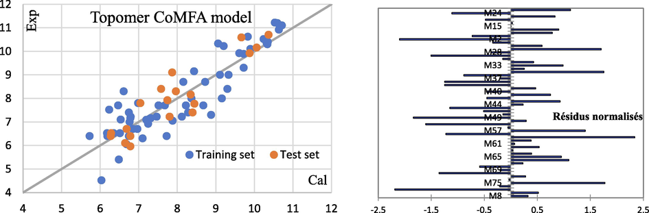
correlation of experimental and predicted values of the Topomer ComFA model and their residues.
3.4.1 Topomer CoMFA contour map analysis
The molecule M65 was chosen to display the contribution of the steric and electrostatic fields represented in Fig. 13.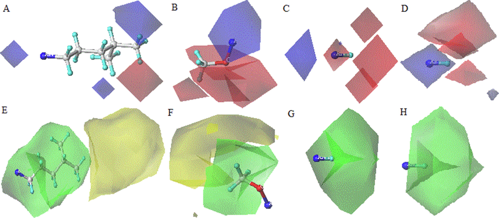
Contour Map Analysis of the Topomer CoMFA Model (A, B, C, and D correspond to the electrostatic fields R1, R2, R3, and R4, respectively) and (E, F, G, and H correspond to the Electrostatic field R1, R2, R3, and R4 respectively).
The generation of contour maps obtained by the Topomer CoMFA model is based on the R1, R2, R3, and R4 fragments, the Topomer CoMFA model shows that it is a significant detection model, Fig 13 represents the contour maps generated around each fragment.
- Electrostatic field: the contribution of the electrostatic field of 80% favorable in blue color around fragment R4, Fig. 13 (D) and 20% unfavorable in red color around fragments R2 and R3, Fig. 13 (B and C) indicate that the addition of an electropositive group in fragment R4 and of an electropositive group in fragments R2 and R3 can be decreases the olfactory threshold of the odorous molecules.
- Steric field: The 80% favorable green steric contribution around the R1, R2, R3, and R4 fragments, represented in Fig. 13 (E, F, G, and H), indicates that adding a bulky group to these fragments can reduce the odor threshold of odorant molecules.
3.5 Validation of prediction models
External Validation Plus 1.2 is a tool that computes all of the essential external validation parameters https://teqip.jdvu.ac.in/QSAR_Tools/, as well as judging the performance of prediction quality of a QSPR model using MAE-based criteria. It can also check for the presence of systematic mistakes in the model.
All calculated external validation parameters (shown in Table 14), along with some basic information about the data structure, are necessary for assessing the quality of QSAR model predictions. We have selected an option regarding the output file will also indicate whether systematic error is present or not, designated as “present” or “absent” based on the 5 conditions mentioned before. It summarizes the information again, all validation parameters are necessary to evaluate the performance of the quality predictive of each QSPR model. Based on these results, it can be observed that the HQSPR and Monte-Carlo (TF2) models are good predictive models.
User Input File Info
File Name
CoMSIA
HQSPR
Tomer CoMFA
TF1
TF2
Model test
Systematic Error Result
Absent
Absent
Absent
Absent
Absent
nPE / nNE
1.429
2.167
1.714
1.714
2.167
nNE / nPE
0.700
0.462
0.583
0.583
0.462
|MPE / MNE|
0.567
1.179
1.090
1.432
2.519
|MNE / MPE|
1.765
0.848
0.917
0.698
0.397
AAE - |AE|
0.595
0.343
0.354
0.488
0.176
(Residuals serial correlation)
0.267
0.212
0.131
0.017
0.058
(Residuals and
values)
0.392
0.333
0.220
0.326
0.219
Classical Metrics (For 100% data)
0.693
0.791
0.840
0.646
0.834
0.690
0.789
0.839
0.643
0.833
0.491
0.714
0.804
0.521
0.809
0.693
0.754
0.829
0.588
0.763
0.688
0.754
0.828
0.588
0.763
0.531
0.719
0.782
0.543
0.772
0.233
0.063
0.056
0.003
0.119
CCC
0.807
0.856
0.904
0.762
0.872
Classical Metric (after removing 5% data with high residuals)
0.744
0.863
0.871
0.749
0.909
0.742
0.857
0.871
0.749
0.908
0.479
0.656
0.730
0.522
0.800
0.751
0.841
0.868
0.649
0.867
0.741
0.840
0.867
0.649
0.866
0.621
0.802
0.824
0.668
0.871
0.195
0.103
0.082
0.043
0.068
CCC
0.844
0.907
0.927
0.798
0.927
Error-based metrics (for 100% data)
0.825
0.734
0.614
0.951
0.721
0.503
0.420
0.356
0.451
0.456
0.122
0.096
0.082
0.104
0.105
0.665
0.610
0.507
0.843
0.568
Error-based metric (after removing 5% data with high residuals)
0.745
0.598
0.546
0.895
0.548
0.450
0.274
0.302
0.417
0.268
0.112
0.065
0.071
0.098
0.063
0.604
0.536
0.461
0.797
0.482
1.953
1.358
1.367
2.049
1.285
BASIC DATA STRUCTURE INFORMATION
Number of test set compounds, Range and Mean (train and test)
NCompTest
17.000
19.000
19.000
19.000
19.000
Train range
7.702
7.700
6.700
7.700
7.700
TrainYMean
7.955
8.000
8.080
8.025
8.025
Test range
4.740
4.740
4.740
4.744
4.744
TestYMean
8.142
7.975
7.975
7.973
7.973
Distribution of observed response values of Test set around Test mean (in %)
35.294
31.579
31.579
31.579
31.579
52.941
42.105
42.105
42.105
42.105
52.941
57.895
57.895
57.895
57.895
70.588
78.947
78.947
78.947
78.947
Distribution of observed response values of Test set around Train mean (in %)
35.294
31.579
31.579
31.579
31.579
47.059
42.105
42.105
42.105
42.105
58.824
57.895
52.632
52.632
52.632
82.353
78.947
78.947
78.947
78.947
Distribution of prediction errors (in %)
%NComp>(0.1*TR)
41.176
26.316
26.316
52.632
21.053
%NComp>(0.15*TR)
23.529
5.263
5.263
21.053
5.263
%NComp>(0.2*TR)
5.882
5.263
0.000
15.789
5.263
%NComp>(0.25*TR)
0.000
5.263
0.000
0.000
5.263
Threshold values utilized to judge the model predictions
(0.1*TrainingSetRange)
0.770
0.770
0.670
0.770
0.770
(0.15*TrainingSetRange)
1.155
1.155
1.005
1.155
1.155
(0.2*TrainingSetRange)
1.540
1.540
1.340
1.540
1.540
(0.25*TrainingSetRange)
1.926
1.925
1.675
1.925
1.925
RESULT (MAE-based criteria applied on 95% data)
Prediction Quality
BAD
GOOD
MODERATE
BAD
GOOD
3.6 Design new compounds
According to the OECD principles, the established QSAR model must be mechanically interpretable, meaning that molecular structural information can be extracted from it. This principle is upheld by the Monte Carlo method, which has revealed optimal molecular descriptors linked directly by molecular fragments.
After recording the numerical data collected during the Monte Carlo optimization cycles, it can be noted that characteristics extracted from SMILES with positive correlation weights in all cycles favor an increase in the final score, while those with negative correlation weights favor a decrease in the parameter in all analyses. The table below lists all the SAk values, as well as the correlation weight values for three Monte Carlo optimization cycles of the QSPR model built. SAk values with a positive value can therefore be classified as promoters of the increase in the log (1/t) value.
On the other hand, SAk with negative values can therefore be classified as a promoter of the decrease in the log (1/t) value. The SAk analysis presented in the Table 15 can be used to guide us in proposing new odorous molecules with a low or high olfactory threshold depending on the chosen promoters.
SAks
CWSAk
ID
NSs
NSc
NSv
Defect [SAk]
Comments
S…C…C…
−2.12
149
2
3
2
0.0013
presence of sulfur and alkyl chain
=…C…1…
−1.75
24
1
2
3
0.0270
Combination of double bond with carbon and carbon ring structure
++++S---B2==
−1.50
10
7
5
8
0.0047
Presence of sulfur with double bond
C…S…(…
2.00
55
4
2
6
0.0116
Combination of sp3 carbon, sp3 sulfur with branching
C…O…(…
2.00
53
5
3
4
0.0044
Combination of sp3 carbon, sp3 oxygen and with branching
N…(….…...
2.06
116
14
12
14
0.0013
Combination of sp3 nitrogen with branching
O…C…1…
2.12
136
3
5
3
0.0013
Combination of sp3 oxygen, sp3 carbon and carbon ring structure
S…(….…...
2.13
142
5
2
6
0.0060
Combination of sp3 sulfur with branching
=…N…1…
2.25
27
20
18
17
0.0028
Combination of double-bonded nitrogen and with carbon ring structure
N…1….…...
2.25
121
20
18
17
0.0028
Combination of sp3 nitrogen connected to carbon ring structure
HALO00000000
2.44
115
20
20
19
0.0000
Absence of fluorine, Chlorine, and Bromine atom
N…(…C…
2.50
118
10
12
11
0.0038
Combination of sp3 nitrogen, branching with to sp3 carbon
C…N… = …
2.56
52
6
9
6
0.0013
Combination of sp3 nitrogen, carbon ring structure with sp3 carbon
C… = …1…
2.56
44
20
18
17
0.0028
Presence of double-bonded carbon with carbon ring structure
N…=…(…
2.63
122
1
1
0
1.0000
Combination of nitrogen with double bond and branching
++++N---B2==
2.75
6
20
20
19
0.0000
Presence of nitrogen with double bond
C…S…C…
2.75
56
2
3
2
0.0013
presence of sp3 carbon connected to sulfur and carbon chain sp3
N… = …C…
2.87
125
20
20
19
0.0000
Presence of double-bonded nitrogen with carbon
S…C…1…
3.06
147
2
3
2
0.0013
Combination of sp3 sulfur, sp3 carbon and carbon ring structure
NOSP10000000
3.19
139
5
5
3
0.0115
presence of heteroatoms
S…C…(…
3.57
145
1
1
2
0.0184
Combination of sp3 sulfur, sp3 carbon and branching
N…C….…...
3.75
127
6
9
6
0.0013
Combination of sp3 nitrogen and sp3 carbon
N…C… = …
3.99
128
6
9
6
0.0013
Combination of nitrogen sp3 and carbon with double bond
N… = ….…...
4.37
123
20
20
19
0.0000
Presence of nitrogen with double bond
N….….......
4.68
119
20
20
19
0.0000
Presence of nitrogen atom
O…C…(…
5.99
134
3
2
2
0.0089
Combination of sp3 oxygen, sp3 carbon and branching
BOND10000000
6.00
58
20
20
19
0.0000
Presence of double bonds and absence of triple and stereochemical bonds
One of the advantages of Monte Carlo simulation is that it provides a much broader view of what might happen. It shows not only what might happen, but to what extent.
This is why we have chosen this method and applied the concepts of Odor Threshold Increase and Odor Threshold Decrease promoters in the TF2 module to propose new odorant molecules, shown in Table 16.

N0
R1
R2
R3
R4
TF1 Model
TF2 Model
HQSAR_59
CoMSIA HES
CoMFA Topomer
P1
(CH2)3CH(CH3)2
OCH3
SC2H5
H
11,2827
13,7811
13.033
9.766
12.730
P2
(CH2)3CH(CH3)2
OCH3
H
SC2H5
10,7003
12,9523
12.755
13.939
12.730
P3
(CH2)3CH(CH3)2
OCH3
SO2H
H
11,3531
11,7579
12.863
11.771
12.870
P4
(CH2)3CH(CH3)2
OCH3
H
SO2H
11,5089
11,0074
12.850
11.373
12.870
P5
(CH2)3CH(CH3)2
OCH3
SO3H
H
11,7104
13,7584
11.248
12.313
13.650
P6
(CH2)3CH(CH3)2
OCH3
H
SO3H
11,8661
13,0079
11.506
10.984
13.650
P7
(CH2)3CH(CH3)2
OCH3
Cl
H
11,1647
11,1793
10.836
13.257
12.320
P8
(CH2)3CH(CH3)2
OCH3
H
Cl
11,3204
10,5141
10.894
11.870
12.320
P9
(CH2)3CH(CH3)2
OCH3
Br
H
11,1647
11,1793
10.894
13.725
12.550
P10
(CH2)3CH(CH3)2
OCH3
H
Br
11,3204
10,5141
10.836
11.862
12.550
P11
(CH2)3CH(CH3)2
OCH3
F
H
11,1647
11,1793
10.836
13.180
11.620
P12
(CH2)3CH(CH3)2
OCH3
H
F
11,3204
10,5141
10.894
10.818
11.720
P13
(CH2)3CH(CH3)2
OCH3
CH2NCH2
H
13,9573
16,4071
11.990
11.865
13.01
P14
(CH2)3CH(CH3)2
OCH3
H
CH2NCH2
14,1131
15,6566
11.915
11.844
13.01
P15
(CH2)3CH(CH3)2
OCH3
NH2
H
11,9319
13,2617
12.871
11.579
12.58
P16
(CH2)3CH(CH3)2
OCH3
H
NH2
12,2101
12,9421
12.110
10.303
12.58
P17
(CH2)3CH(CH3)2
OCH3
CH2SCH3
H
12,5228
15,2256
13.548
9.087
13.14
P18
(CH2)3CH(CH3)2
OCH3
H
CH2SCH3
12,6785
14,4751
12.577
11.062
13.14
P19
(CH2)3CH(CH3)2
OCH3
NCH2
H
14,1224
16,7947
11.255
12.263
13.18
P20
(CH2)3CH(CH3)2
OCH3
H
NCH2
13,7986
15,6984
11.043
11.780
13.18
P21
(CH2)3CH(CH3)2
OCH3
N2H
H
13,2396
16,8977
10.718
13.998
12.59
P22
(CH2)3CH(CH3)2
OCH3
H
N2H
13,1926
15,7491
10.875
11.446
12.59
P23
(CH2)3CH(CH3)2
OCH3
OH
H
11,4706
12,0438
12.038
12.508
12.59
24
(CH2)3CH(CH3)2
OCH3
H
OH
11,6264
11,6115
12.578
12.736
12.28
P25
(CH2)3CH(CH3)2
OCH3
SH
H
11,2870
11,9595
12.038
12.863
13.52
P26
(CH2)3CH(CH3)2
OCH3
H
SH
11,4427
11,3121
12.578
10.757
13.52
P27
(CH2)3CH(CH3)2
OCH3
NHCH3
H
12,1006
15,6449
13.425
12.355
13.04
P28
(CH2)3CH(CH3)2
OCH3
H
NHCH3
11,5183
14,8161
12.578
11.464
13.04
P29
(CH2)3CH(CH3)2
OCH3
NHCHCH2
H
13,4120
16,6750
14.048
11.938
13.10
P30
(CH2)3CH(CH3)2
OCH3
H
NHCHCH2
13,5678
15,9245
13.124
12.105
13.10
P31
(CH2)3CH(CH3)2
OCH3
NHC2H5
H
12,0440
15,4821
13.981
12.463
13.08
P32
(CH2)3CH(CH3)2
OCH3
H
NHC2H5
11,4617
14,6533
13.330
12.233
13.08
P33
(CH2)3CH(CH3)2
OCH3
CHCHCH3
H
12,5707
13,8828
12.298
11.973
12.52
P34
(CH2)3CH(CH3)2
OCH3
H
CHCHCH3
12,7265
13,1323
12.019
11.913
12.52
P35
(CH2)3CH(CH3)2
OCH3
SCH3
H
12,4852
14,7945
13.487
12.107
12.71
P36
(CH2)3CH(CH3)2
OCH3
H
SCH3
12,6409
14,0440
13.284
12.827
12.71
All proposals from Monte-Carlo TF2 model promoters have decreased the olfactory threshold except for the presence of halogens which will increase the olfactory threshold value. According to the prediction values, we verified these proposals using the HQSPR method and found that the two models are closer at the prediction levels.
3.7 Molecular docking results
The porcine odorant-binding protein (pOBP) has been chosen as a simple model for Molecular Docking of odorant molecules, the choice of the 1DZK.pdb protein is based on the reference ligand (2-methoxy-3-(2-methylpropyl) pyrazine noted M63) which has already been mentioned previously of this protein. Specifically, we used chain B at two attack positions P1 and P2. The analysis of this crystalline structure at a resolution of less than 2 Å and a R factor not exceeding 20%, a good quality model should have more than 90% in the most favored regions [A, B, L]. The lengths and ϕ and ψ bond angles of the main chain are compared to the ideal values of derived from small molecule data(Ravikumar et al., 2019). Therefore, structures refined using different constraints may show apparently large deviations from normality, which are shown in the following Fig 14.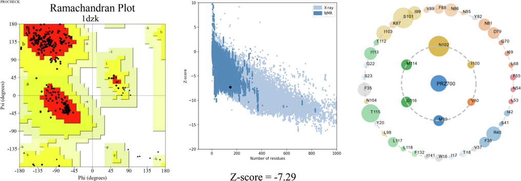
Ramachandran plot, Screenshot of ProSA-web used to confirm protein structure and active sites of protein 1DZK chains: B.
The absence of outliers during the analysis of phi (φ) and psi (ψ) torsion nails of the residues (amino acids) of this crystal structure shows that this combination of angles is possible and a negative Z-score indicates the overall quality of the model. After the confirmation of the crystal structure, we displayed that the active residues of the B-chain such as ASN:102, MTE:114, GLY:116, MET:39, VAL:80 and ILE:100 are odor transporter keywords.
We used several available Molecular Docking software to choose the program that gives reliable results and to give a clear overview of the affinity of the studied complexes. We started with methoxypyrazine-based ligands from the database, which are represented in the following Table 17. *Reference Ligand for Proteine 1DZK.
Ligands
AM-Dock
Autodock-Vina
Pyrex
Sybyl
Ligands
AM-Dock
Autodock-Vina
Pyrex
Sybyl
M12
−4.9
−4.9
−5.0
2.762
M58
−6.83
−7.8
−7.8
5.196
M18
−3.78
−4.8
−5.0
2.671
M59
−5.47
−6.7
−6.7
4.495
M49
−3.45
−4.3
−4.2
3.295
M60
−5,24
−6.4
−6.4
4.653
M50
−3.90
−5.0
−5.1
3.549
M61
−5.08
−6.1
−6.1
4.287
M51
−4.28
−5.3
−5.4
3.791
M62
−5.73
−7.0
−6.9
4.871
M52
−4.55
−5.7
−5.8
3.618
M63*
−5.04
−6.2
−6.2
3.585
M53
−4.93
−6.0
−6.0
3.896
M64
−5.42
−6.6
−6.6
3.798
M54
−5.34
−6.4
−6.4
5.548
M65
−5.83
−6.9
−7.1
5.096
M55
−5.66
−6.7
−6.7
5.185
M66
−4.77
−5.8
−5.9
3.472
M56
−5.91
−7.0
−6.9
5.538
M67
−5.51
−6.8
−6.8
5.156
M57
−6.31
−7.4
−7.4
5.721
M68
−5.7
−6.8
−6.8
5.088
The results of the Molecular Docking process are influenced by the algorithms used in each program and the method of execution (such as automatic with AM-Dock, position P1 and dimensions (30) with Autodock-vina, position P1 and dimension based on ligand volume with Peryx, and active residue selection with Sybyl). Our observations show that Autodock-vina and Peryx produce the most accurate and effective results. The affinity of the complexes can vary based on the number of carbon atoms in fragment R2, which has been depicted in a correlative Fig. 15.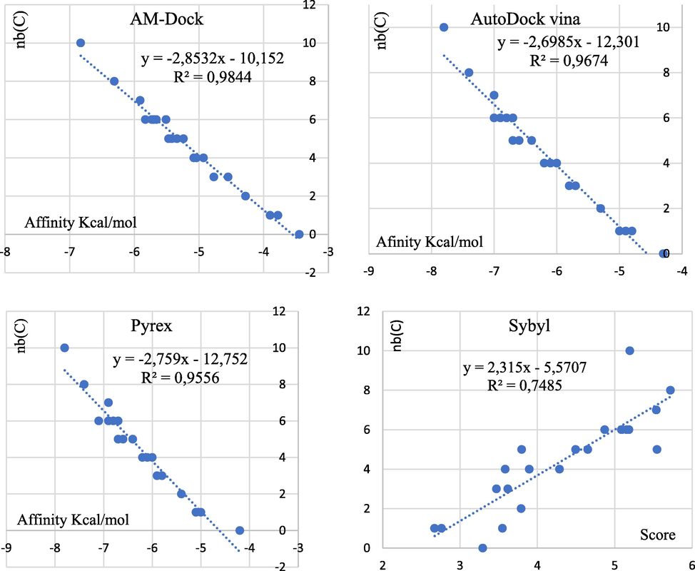
The correlation between the number of fragment carbon R2 and complex affinity.
The four programs employed were used to describe the relation of the affinities and carbon number of the hydrophilic substituents in position R1 (CoMSIA/SEH) and the steric action (topomer-CoMFA) of the fragment.
3.7.1 Re-docking results
The results of ligand superposition illustrated in Fig. 16, before and after Molecular Docking show that the P1 position gives more reliable results than P2 according to the RSMD values of Autodock-vina, the other software gives values higher than these values.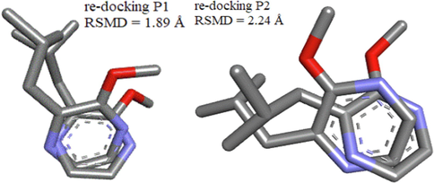
Redocking of the active site positions (P1) and (P2) with the RMSD values.
We selected the Autodock-vina program to perform molecular docking at the (P1) coordinates of the proposed molecules, based on the results of redocking. The affinity results are shown in the following Table 18 and the visualization of interactions are shown in Fig. 17.
-
Interactions of compound M63
| Ligands | Affinity Kcal/mol | Ligands | Affinity Kcal/mol | Ligands | Affinity Kcal/mol | Ligands | Affinity Kcal/mol | Ligands | Affinity Kcal/mol | Ligands | Affinity Kcal/mol |
|---|---|---|---|---|---|---|---|---|---|---|---|
| P1 | −7.5 | P7 | −7.5 | P13 | −7.4 | P19 | −7.4 | P25 | −7.2 | P31 | −7.2 |
| P2 | −6.9 | P8 | −7.3 | P14 | −7.3 | P20 | −7.4 | P26 | −6.9 | P32 | −7.2 |
| P3 | −7.7 | P9 | −7.6 | P15 | −7.2 | P21 | −7.7 | P26 | −7.2 | P33 | −7.0 |
| P4 | −7.7 | P10 | −7.4 | P16 | −7.5 | P22 | −7.8 | P28 | −7.4 | P34 | −7.0 |
| P5 | −7.7 | P11 | −7.5 | P17 | −7.4 | P23 | −7.3 | P27 | −7.4 | P35 | −7.4 |
| P6 | −7.5 | P12 | −7.7 | P18 | −6.7 | P24 | −7.4 | P30 | −6.8 | P36 | −7.3 |
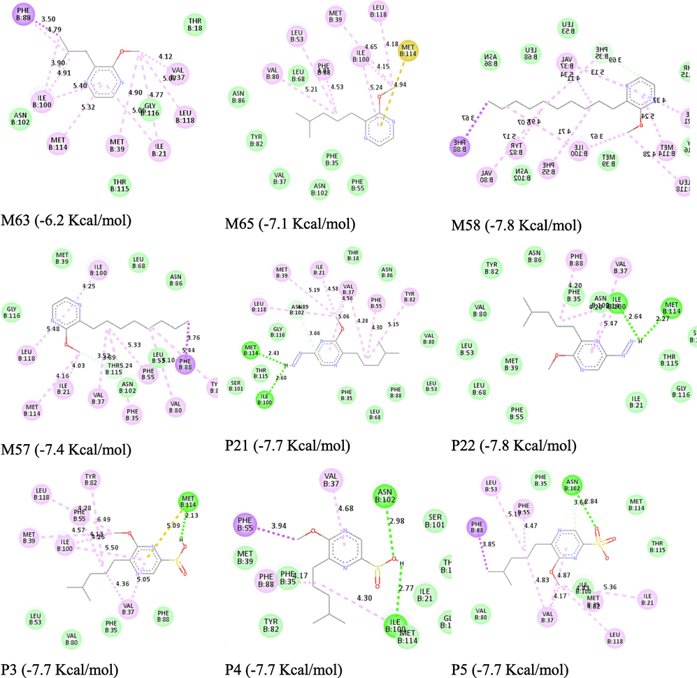
- The interactions of newly designed compounds are shown in 2D docking poses.
The compound M63 is a reference ligand for the protein 1DZK.pdb. It formed pi-sigma interactions of about 3.5 Å between the aromatic of the amino acid PHE:88 and the isopropyl carbon. It also formed three pi-alkyl bonds, one with the same amino acid at 4.9 Å and two with ILE:100 at 3.9 Å and 4.91 Å. The methoxy group of fragments R2 formed three bonds with the residues VAL:37 (4.12 Å), MET:39 (4.9 Å), and LEU:118 (5.08 Å). The common pyrazine structure also involves pi-alkyl interactions with the ILE:100 amino acid at 5.4 Å and MET:114 at 5.32 Å. Although these interactions are weaker than hydrogen bonds, they are still important for odor transport, except for the amino acid PHE:88.
-
Interactions of compound M65
The M65 complex formed pi-sulfur interactions between the amino acid MET:114 and the common pyrazine ring structure at a distance of 4.94 Å, while other interactions were pi-Alkyl type such as MET:39 (4.65 Å), ILE:100 (5.24 Å, 4.15 Å) and VAL:80 (5.21 Å). However, the branching of the R1 fragment decreases the olfactory threshold and these interactions are weaker than hydrogen bonds, making this complex's affinity smaller than that of the reference ligand, meaning that the odor transduction of this molecule is possible.
-
Interactions of compound M57
The M57 compound formed non-classical hydrogen type interactions between the oxygen of the aldehyde functional group of the amino acid THR:115 specifically the non-bonding oxygen doublet and the R2 fragment of the methoxy group with a distance of 3.52 Å, unfortunately the amino acid THR:115 does not belong to the odor transporters keywords of the protein 1DZK.pdb (chain B). Other remarkable interactions as keywords formed a pi-sigma type bond between the ring of the amino acid PHE:88 and carbon number 8 of the R1 fragment at a distance of 3.76 Å. However, other amino acids VAL:80, ILE:100, and MET:114 formed pi-Alkyl type bonds with distances of 5.10 Å, 4.25 Å, and 4.16 Å respectively.
-
Interactions of compound M58
The M58 compound formed non-classical hydrogen type interactions between carbon number 5 of the common pyrazine structure and the non-bonding oxygen doublet of the aldehyde functional group of amino acid PHE:35 at a distance of 3.69 Å and a pi-Alkyl type bond with the linear chain of the R1 fragment at a distance of 4.11 Å, unfortunately the amino acid PHE:35 does not belong to the odor transporter keywords of protein 1DZK.pdb (chain B). Other remarkable interactions as keywords formed a pi-sigma type bond between the ring of amino acid PHE:88 and carbon number 10 of the R1 fragment at a distance of 3.76 Å. However, other amino acids VAL:80, ILE:100, and MET:114 formed pi-Alkyl type bonds with distances of 5.17 Å, 3.67 Å, and 5.24 Å respectively.
-
Interactions of compound P21
The compound P21 formed hydrogen bond interactions between the carbon number 5 of the pyrazine structure and the non-bonding oxygen doublet of the amide function of the amino acid ASN:102 at a distance of 3.66 Å, and another conventional hydrogen bond between the diazene hydrogen of the R3 fragment and the non-bonding oxygen doublets of the aldehyde function of the amino acids MET:114 and ILE:100 at a distance of 2.43 Å and 2.6 Å, respectively. Although the addition of diazenyl in the R3 position decreases the olfactory threshold, this fragment contributes to attaching the compound P11/R3 during the transduction of the smell of this molecule.
-
Interactions of compound P22
The compound P22 forms two conventional hydrogen bond interactions between the diazene hydrogen of the R3 fragment and the non-bonding double bonds of the oxygen atoms of the aldehyde function of the amino acids MET:114 and ILE:100 at a distance of 2.27 Å and 2.64 Å respectively. On the other hand, there are three pi-Alkyl type bonds, two bonds between the amino acid ILE:100, one with the R1 fragment at a distance of 4.2 Å, and the other with the pyrazine structure common ring, and another bond between the amino acid PHE:88 and the R1 fragment at a distance of 4.2 Å. Although the addition of diazenyl at R4 position decreases the odor threshold, it contributes to binding the compound P11/R4 during odor transduction of this molecule.
-
Interactions of compound P3
The compound P3 forms important conventional hydrogen bond interactions at a distance of 2.13 Å between the non-bonding double bond of the oxygen atom of the aldehyde function of the amino acid MET:114 and the sulfinic substitution hydrogen of the R3 fragment and pi-sulfur type with the same amino acid at a distance of 5.09 Å. Other interactions are formed of pi-Alkyl type such as ILE:100 and the common pyrazine structure at a distance of 5.5 Å and between the methoxy substitution of the R2 fragment with the amino acids MET:39 and ILE:100 at a distance of 4.57 Å, 4.26 Å respectively.
-
Interactions of compound P4
The compound P4 forms conventional hydrogen bond interactions between the primary amine hydrogen atom of the amino acid ASN:102 and the non-bonding double bond of the sulfinic acid oxygen atom at a distance of 2.98 Å, another interaction between the sulfinic acid hydrogen and the non-bonding double bond of the oxygen atom of the aldehyde function of the amino acid ILE:100 at a distance of 2.77 Å, another pi-Alkyl type bond of a distance of 4.3 Å between the previous amino acid ILE:100 and the R1 fragment. These interactions that we mentioned may be key factors in the odor transduction of this molecule.
-
Interactions of compound P5
The compound P5 forms conventional hydrogen bond interactions between the non-bonding double bond of the sulfonic acid oxygen atom and the primary amine hydrogen of the amino acid ASN:102 at a distance of 2.84 Å, and a carbon-hydrogen bond between the non-bonding double bond of the oxygen atom of the amide function of the same amino acid and the carbon hydrogen number 5 of the common pyrazine structure. Another pi-Alkyl bond is formed between the amino acid MET:39 and the methoxy substitution of the R2 fragment at a distance of 4.43 Å. It should be noted that other interactions such as a pi-sigma bond of the amino acid PHE:88 and various pi-Alkyl bonds with other amino acids influenced the affinity of this compound, but these residues do not belong to the set of odor transduction keywords.
3.8 ADME-Tox results
The pharmacokinetic properties show (Table 19) that all compounds are non-toxic, confirming the Lipinski rules. The logBB values are in the range [-1; 0.3], indicating that all the compounds are poorly diffused in the brain, with a solubility in octanol preferable to water, and a synthesis accessibility in the range [1; 10]. None of the candidate molecules inhibit the enzymes involved in the metabolic pathway.
Property
M65
M63
M58
M57
P21
P22
P3
P4
P5
Absorption (%)
95.95
97.05
94.75
95.44
90.64
90.45
92.84
92.86
91.07
logBB
0.05
−0.11
0.22
0.30
−0.40
−0.36
−0.62
−0.60
−0.82
CYP2D6
No
No
No
No
No
No
No
No
No
CYP 3A1
No
No
Yes
No
No
No
No
No
No
CYP1A2
Yes
Yes
Yes
Yes
Yes
Yes
No
No
No
CYP2C19
No
No
Yes
No
No
No
No
No
No
CYP2C9
No
No
No
No
No
No
No
No
No
CYP2D6
No
No
No
No
No
No
No
No
No
CYP3A4
No
No
No
No
No
No
No
No
No
Total clearance (log ml/min/kg)
0.76
0.74
1.69
1.63
0.45
0.65
0.68
0.16
1.10
AMES toxicity
No
No
No
No
No
No
No
No
No
Synthetic acceessibility
2.81
2.57
3.24
3.03
3.20
3.20
3.48
3.60
3.36
LogP
3.68
2.62
5.99
4.93
3.64
3.35
2.17
2.37
3.19
NRB
5
3
10
8
6
6
6
6
6
NHA
3
3
3
3
5
5
5
5
6
NHD
0
0
0
0
1
1
1
1
1
MW (Dalton)
194.3
166.2
250.4
222.3
222.3
222.3
258.3
258.3
290.4
TPSA (Å2)
35.01
35.01
35.01
35.01
71.22
71.22
91.52
91.52
97.96
3.9 Analyzing the binding stability of protein–ligand interactions during MD simulations
The stability of the top complexes was assessed by performing MD calculations during 100 ns simulations under ambient temperature conditions. Visualization of the trajectories after running the simulations showed that all ligands remained stable within the protein binding pocket. Calculations of RMSD, RMSF, gyration radius, hydrogen bonding, medium mass center (COM) distance between the protein and ligands, and binding free energy (MMPBSA) were performed to assess the stability of each complex.
The RMSD plots in Fig. 18 show the RMSD of the complex, protein backbone and ligand for each structure. The RMSD of the protein backbone and complex remained stable and below 2 Å after 10 ns of simulation.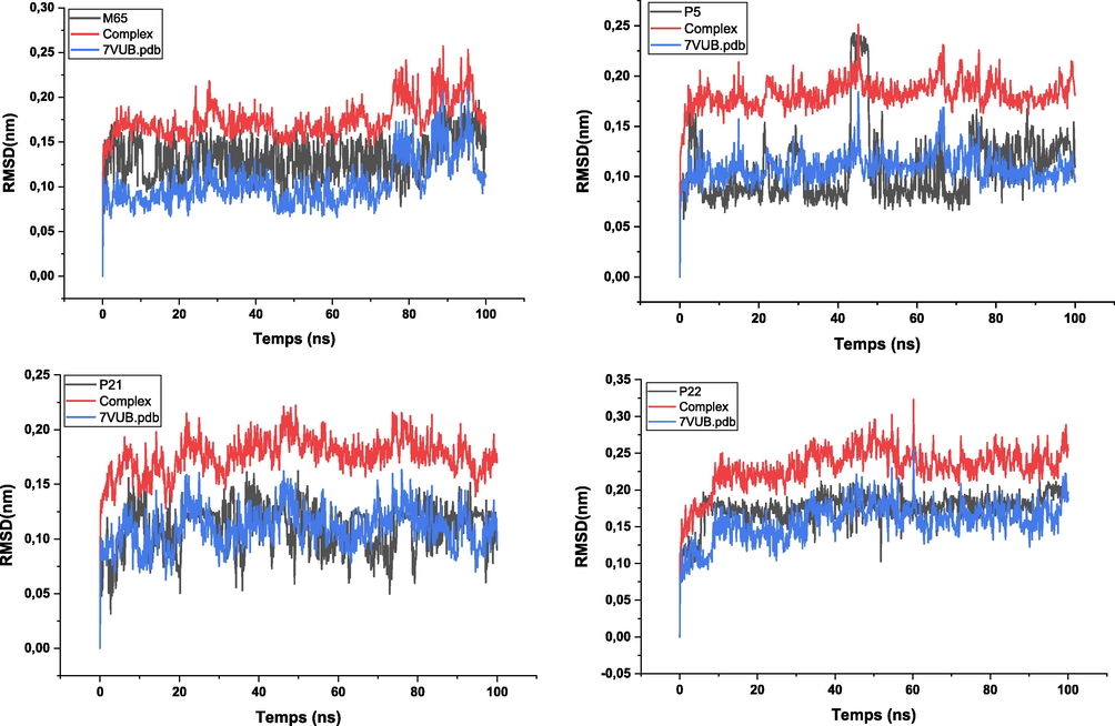
RMSD values of the complexes during 100 ns of MD simulations.
The RMSF was calculated for the protein complex using GROMACS, focusing on the C-alpha atoms. Overall, the size of the fluctuations remains below 2.0 Å for all compounds, except for certain residues that form loops or turns in the protein (Fig. 19). Similar behaviors were observed for the RMSF, but with different intensities for each ligand. Ligand P22 showed significantly higher fluctuations between the ranges (20–36) ns, (75–85) ns and (104–112) ns, but still below 3.07 Å. On the other hand, the fluctuations of ligand P5 were consistently lower compared to the other ligands.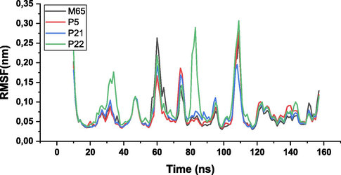
RMSF values of the complexes during 100 ns of MD simulations.
Analysis of the radius of gyration (Fig. 20) shows high stability for all complexes, with very low overall fluctuations and fluctuations along the Y and Z axes of less than 1.25 nm. This indicates the compactness and stability of the protein–ligand system. However, in terms of the radius of gyration along the X axis, we observed values between 1.45 nm and 1.50 nm throughout the dynamic simulation, indicating significant atomic vibration along this axis. This finding suggests that there is a pronounced motion or flexibility in the X-axis direction, which may be due to specific residues or structural features of the protein–ligand complex. It is important to further investigate the cause of this increased oscillation and its potential impact on the stability and binding affinity of the complex. Additional analysis, such as examining the local environment and interactions in this region, may provide insight into the structural dynamics and functional implications of the observed fluctuations.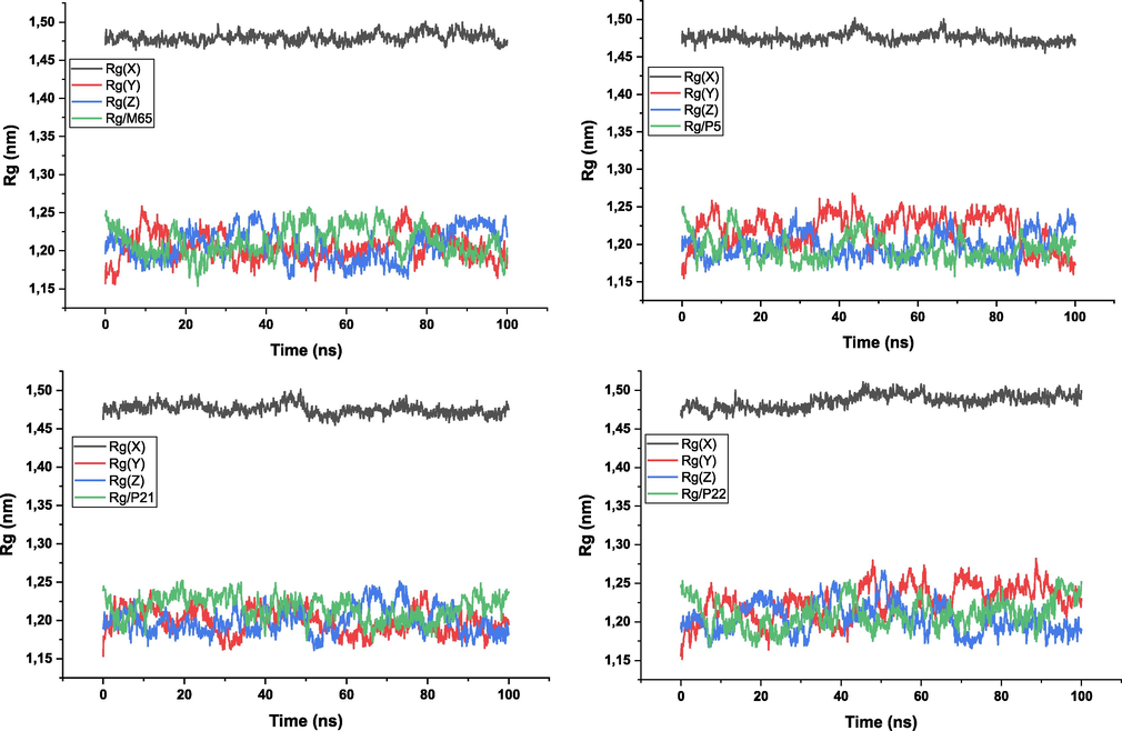
Radius of gyration values of the complexes during 100 ns of MD simulations.
The total number of hydrogen bonds formed between the ligand and the protein during the 100 ns simulation is presented in Fig. 21. The P5 and P21 ligands have a higher number of hydrogen bonds compared to M65, which formed only one hydrogen bond throughout the simulation. In addition, the P22 ligand formed discontinuous hydrogen bonds with the protein, ranging from zero to three hydrogen bonds, with an average of one hydrogen bond over the entire simulation.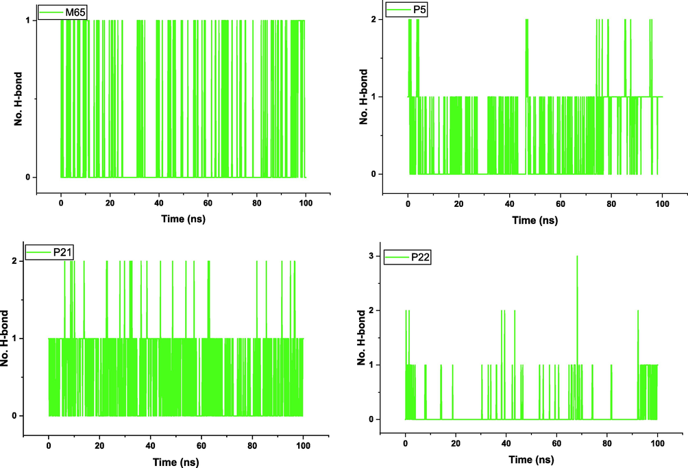
Number of hydrogen bonds (protein–ligand) for the complexes during 100 ns of MD simulation.
It is interesting to note that the P5 and P21 ligands also formed several non-hydrogen interactions, Fig. 22 with respectively up to six and eight of these interactions, at distances comparable to those of a hydrogen bond throughout the simulation. This suggests that the stabilizing interaction between the ligand and the protein is of a different nature, possibly involving other types of non-covalent interactions such as hydrophobic interactions or pi-stacking. These additional interactions contribute to the overall stability and binding affinity of complexes.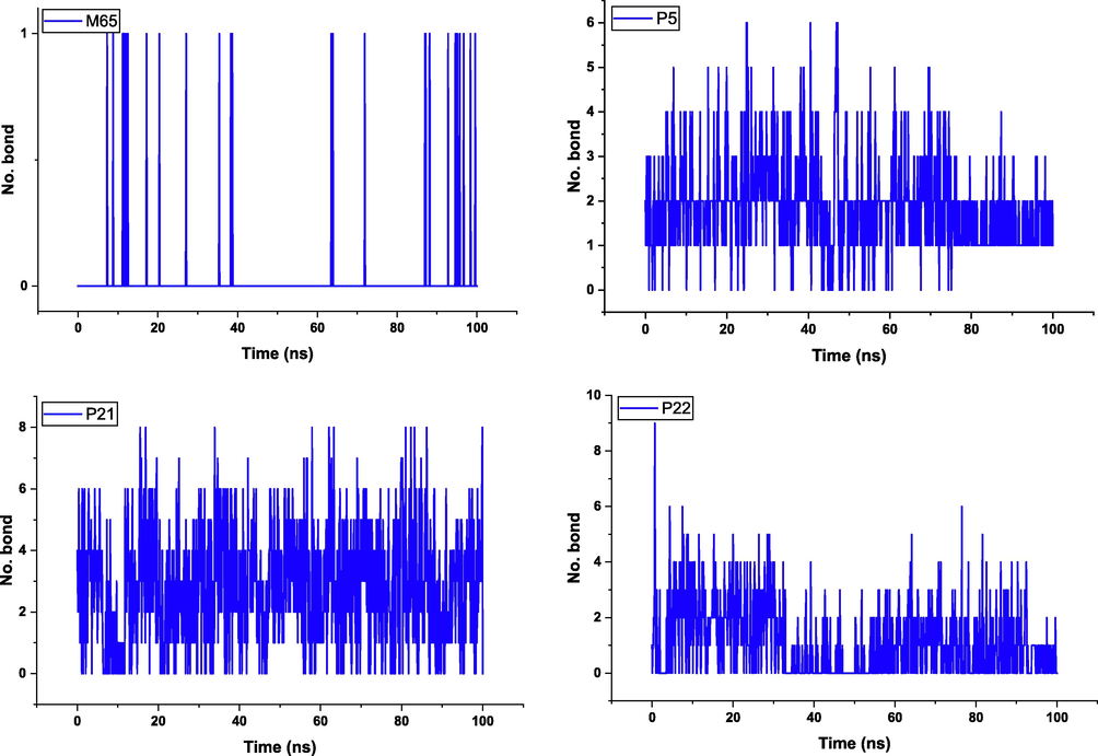
Number of bonds (protein–ligand) for the complexes during 100 ns of MD simulation.
The COM distance shown in Fig. 23 remains relatively stable for the three investigated complexes, with variations of about 0.34 nm for M65, 0.37 nm for P5, 0.4 nm for P21 and 0.75 nm for P22.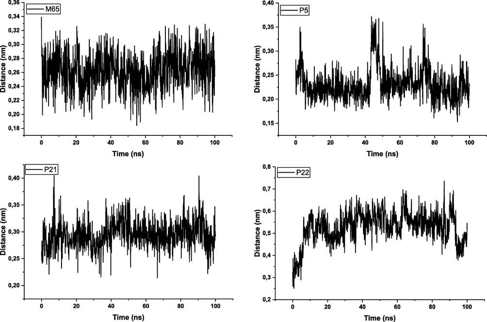
COM distance of complexes during 100 ns of MD simulation.
These values indicate the average distance between the center of mass of the ligand and the protein during the simulation. A stable and constant COM distance indicates that the ligand maintains a good affinity with the protein binding pocket throughout the simulation. For M65, the COM distance remains relatively constant, indicating stability and regular interaction with the protein.
However, slight fluctuations are observed for the P5, P21 and P22 ligands, which may be due to dynamic motions or conformational changes of the protein or ligand during the simulation. These fluctuations may reflect conformational adjustments necessary to maintain a stable ligand–protein interaction.
It is important to note that although fluctuations in the COM distance are present, they generally remain within a relatively small range. This suggests that the overall stability and interaction of the protein–ligand complexes studied is maintained for the duration of the simulation.
COM distance analysis provides valuable information about the dynamic properties of the protein–ligand bond and the flexibility of the complexes. Understanding these fluctuations and their structural implications can contribute to a better understanding of molecular interactions and the design of more stable and effective ligands.
The potential energy, pressure and temperature of the system during the 100n MD simulation, obtained from the GROMACS edr file, are shown in Fig. 24. The graph shows a potential energy, pressure and temperature converging over the 100 ns simulations. The Molecular Mechanics/Surface Poisson-Boltzmann (MM/PBSA) method was chosen for the re-evaluation of the complexes because it is the fastest force-field based method for calculating the free energy bond, compared to other free energy calculation methods such as Free Energy Perturbation (FEP) or Thermodynamic Integration (TI) methods. The MM/PBSA calculation was performed using the g-mmpbsa software. The calculated free energies of the compounds are shown in Table 20.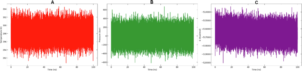
From left to right: (A) Temperature, (B) pressure and (C) potential energy during the 100 ns MD simulations.
Complex
Binding
Van der Waal energy
Electrostatic energy
Polar solvation energy
SASA energy
M65
−111.58 ± 9.55
−132.82 ± 6.72
−13.12 ± 9.21
48.65 ± 5.68
−14.30 ± 0.58
P5
−132.14 ± 7.49
−165.60 ± 8.71
−29.99 ± 8.98
80.18 ± 8.26
−16.74 ± 0.80
P21
−100.15 ± 4.33
−154.86 ± 7.23
−21.05 ± 5.29
91.14 ± 3.76
−15.38 ± 0.75
P22
−83.38 ± 18.45
−133.37 ± 13.89
−24.19 ± 20.85
89.89 ± 14.50
−15.71 ± 0.80
Gibbs free energy is a measure of the overall stability of a complex and a more negative G value indicates greater stability. It can be seen that P5 has the highest free energy, indicating greater stability compared to the other molecules. M65 and P21 also have negative values, but lower ones, while P22 has the lowest value among the others, indicating a relatively lower stability. The Van der Waals energy represents the ligand–protein interaction through Van der Waals forces, which are attractive and repulsive forces. Negative values indicate attraction and positive values repulsion. In this case it can be seen that P5 has the highest Van der Waals energy, indicating a greater attraction between this ligand and the amino acids.
The electrostatic energy measures the electrostatic interaction between the ligand and the surrounding amino acids. It can be observed that ligand P5 has the highest electrostatic energy, indicating greater ligand–protein attraction. The polar solvation energy is the energy required to dissolve the solute (ligand) in a polar solvent. Negative values indicate better solubility as they indicate the release of energy during dissolution. Comparing the values, it can be seen that P21 has the highest polar solvation energy, indicating a relatively lower solubility compared to the other ligands.
The solute accessible surface energy represents the energy of interaction between the ligand and the solvent at the surface of the ligand. Negative values indicate attraction and positive values repulsion. Comparing the absolute values, it can be seen that P5 has the highest solute accessible surface energy, indicating greater attraction between the molecule and the solvent at its surface.
From the data provided it can be concluded that P5 appears to be the most stable molecule, while P21 has a relatively lower solubility and greater attraction to the solvent on its surface. M65 and P22 fall between these two extremes in terms of the properties evaluated.
4 Conclusion
Heterocyclic compounds based on pyrazine have been used for the study of odorous properties by various QSPR methods. Recently, many works have been devoted to the preparation of these compounds and their application for therapeutic, food, cosmetic, and photovoltaic purposes. it should be noted that the molecules containing a 1,4-pyrazine ring can easily be functionalized by addition or substitution on the different positions of the pyrazine ring leading to new functional molecules, which constitutes the chemical importance of these compounds.
We noticed that unfortunately few works in the literature describe the QSPR analysis to predict the olfactory threshold of molecules of this type. For these reasons, we sought an easy, applicable, and reliable way to study this phenomenon. For this purpose, we have chosen the olfactory threshold as an independent variable to study the structure/odor relationship of these molecules using the following techniques:
The Monte Carlo method is based on the SMILE representation of the odorous studied molecules. indeed, the purpose of using this method is to determine and highlight the promoters making it possible to increase and/or decrease the olfactory threshold. the resulting extracted model (TF2), which met all internal and external validation criteria, was successfully obtained.
The HQSPR Method, based on the study of molecular fragments, lets us point out that the advantage of this method is that it does not require molecular alignment and it allows the automatic analysis of large sets of data without manual intervention. This method gives good and reliable results. Although it is a 2D method, it gives precise information about the atoms that contribute significantly to the odor threshold, the final obtained HQSPR (B/C) model met all internal and external validation criteria.
In this work, other 3D-QSPR methods were used, notably the CoMSIA/SEH and Topomer CoMFA models to confirm the results obtained by the previous techniques. These results provided imploring and predictive insight into the nature of the relationship between chemical structure and odor properties.
The results obtained by the 2D-QSPR and 3D-QSPR techniques in our work can be successfully used to predict the required properties and olfactory threshold of various related compounds. They also make it possible to design and screen various odorant molecules, avoiding extensive and costly experimental analyses for less potent molecules. In addition, the compounds P5, P21 and P22 proposed, have formed strong interactions with porcine odor-binding protein (pOBP) located in the pOBP beta-barrel cavity and were stable during dynamic simulation time and had good pharmacokinetic properties.
Declaration of Competing Interest
The authors declare that they have no known competing financial interests or personal relationships that could have appeared to influence the work reported in this paper.
References
- Organic compounds based on 1-(prop-2-yn-1-ylamino)-2,3-dihydro-1H-indene-4-thiol as selective human monoamine oxidase B inhibitors. Quantitative analysis of structure-activity relationships and in-silico investigations. J. Chem.. 2023;2023:802-817.
- [CrossRef] [Google Scholar]
- Structure-based virtual screening and molecular dynamics of phytochemicals derived from Saudi medicinal plants to identify potential COVID-19 therapeutics. Arab. J. Chem.. 2020;13:7224-7234.
- [CrossRef] [Google Scholar]
- 3D-QSAR, docking, molecular dynamics simulation and free energy calculation studies of some pyrimidine derivatives as novel JAK3 inhibitors. Arab. J. Chem.. 2020;13:1052-1078.
- [CrossRef] [Google Scholar]
- 2D-QSPR study of olfactive thresholds for pyrazine derivatives using DFT and statistical methods. Emerg. Sci. J.. 2019;3:179-186.
- [CrossRef] [Google Scholar]
- Chtita, S., Lakhlifi, T., Bouachrine, M, Belhassan, A., Bouachrine, Mohammed, 2018. 3D-QSPR studies of olfactive property for pyrazine derivatives 3D-QSPR studies of olfactive property for pyrazine derivatives MOTS-CLÉS, Proceedings BIOSUNE.
- Computational investigation of novel pyrimidine derivatives as potent FAK inhibitors via 3D-QSAR, molecular docking, molecular dynamics simulation and retrosynthesis. New J. Chem. 2023
- [CrossRef] [Google Scholar]
- Elbouhi, M.H., Ouabane, M., Koubi, Y., Lakhlifi, T., 2022. RHAZES : Green and Applied Chemistry Anti-Tumor Activity of Novel Benzimidazole-Chalcone Hybrids as non-Intercalative Topoisomerase II Catalytic Inhibitors : 2D- QSAR study. https://doi.org/10.48419/IMIST.PRSM/rhazes-v14.31147.
- High-throughput virtual screening approach of natural compounds as target inhibitors of plasmepsin-II. J. Biomol. Struct. Dyn. 2022
- [CrossRef] [Google Scholar]
- Catastrophic collision between obesity and COVID-19 have evoked the computational chemistry for research in silico design of new camkkii inhibitors against obesity by using 3D-QSAR, molecular docking, and ADMET. Orbital. 2021;13:316-327.
- [CrossRef] [Google Scholar]
- Hajji, H., Tabti, K., En-Nahli, F., Bouamrane, S., Lakhlifi, T., Ajana, M.A., Bouachrine, M., 2021b. In Silico Investigation on the Beneficial Effects of Medicinal Plants on Diabetes and Obesity: Molecular Docking, Molecular Dynamic Simulations, and ADMET Studies. https://doi.org/10.33263/BRIAC115.69336949.
- Computational study of quinoline-based thiadiazole compounds as potential antileishmanial inhibitors. New J. Chem.. 2022;46:17554-17576.
- [CrossRef] [Google Scholar]
- A computational study of Di-substituted 1,2,3-triazole derivatives as potential drug candidates against Mycobacterium tuberculosis : 3D-QSAR, molecular docking, molecular dynamics, and ADMETox. New J. Chem.. 2023;47:11832-11841.
- [CrossRef] [Google Scholar]
- Monte Carlo method and GA-MLR-based QSAR modeling of NS5A inhibitors against the Hepatitis C virus. Molecules. 2022;27
- [CrossRef] [Google Scholar]
- Ma, X., 2022. Development of Computational Chemistry and Application of Computational Methods, in: Journal of Physics: Conference Series. Institute of Physics. https://doi.org/10.1088/1742-6596/2386/1/012005.
- In search of novel inhibitors of anti-cancer drug target fibroblast growth factor receptors: Insights from virtual screening, molecular docking, and molecular dynamics: In search of novel inhibitors of anti-cancer drug target fibroblast growth factor receptors. Arab. J. Chem.. 2022;15
- [CrossRef] [Google Scholar]
- Mahmud, S., Biswas, S., Kumar Paul, G., Mita, M.A., Afrose, S., Robiul Hasan, M., Sharmin Sultana Shimu, M., Uddin, M.A.R., Salah Uddin, M., Zaman, S., Kaderi Kibria, K.M., Arif Khan, M., Bin Emran, T., Abu Saleh, M., 2021. Antiviral peptides against the main protease of SARS-CoV-2: A molecular docking and dynamics study. Arabian Journal of Chemistry 14. https://doi.org/10.1016/j.arabjc.2021.103315.
- Pyrazines: Synthesis and industrial application of these valuable flavor and fragrance compounds. Biotechnol. J. 2020
- [CrossRef] [Google Scholar]
- Ong, K.T., Liu, Z.-Q., Meng, &, Tay, G., 2017. Review on the Synthesis of Pyrazine and Its Derivatives, Borneo Journal of Resource Science and Technology.
- Ouabane, M., Hajji, H., Belhassan, A., 2022. RHAZES : Green and Applied Chemistry molecules in pectin gels of different concentration. RHAZES: Green and Applied Chemistry. https://doi.org/10.48419/IMIST.PRSM/rhazes-v14.31151.
- Stereochemical assessment of (φ, ψ) outliers in protein structures using bond Geometry-Specific Ramachandran Steric-Maps. Structure. 2019;27:1875-1884.e2.
- [CrossRef] [Google Scholar]
- The novel 4-hydroxyphenylpyruvate dioxygenase inhibitors in vivo and in silico approach: 3D-QSAR analysis, molecular docking, bioassay and molecular dynamics. Arab. J. Chem.. 2022;15
- [CrossRef] [Google Scholar]
- Tabti, K., el Mchichi, L., Moukhliss, Y., Singh, G., Sbai, A., maghat, H., bouachrine, M., Lakhlifi, T., 2022a. CoMFA Topomer, CoMFA, CoMSIA, HQSAR, docking molecular, dynamique study and ADMET study on phenyloxylpropyl isoxazole derivatives for coxsackie virus B3 virus inhibitors activity. Moroccan Journal of Chemistry 10, 703–725. https://doi.org/10.48317/IMIST.PRSM/morjchem-v10i4.34319.
- Tabti, K., Elmchichi, L., Sbai, A., Maghat, H., Bouachrine, M., Lakhlifi, T., 2022b. Molecular modelling of antiproliferative inhibitors based on SMILES descriptors using Monte-Carlo method, docking, MD simulations and ADME/Tox studies. Mol Simul. https://doi.org/10.1080/08927022.2022.2110246.
- Tabti, K., Elmchichi, L., Sbai, A., Maghat, H., Bouachrine, M., Lakhlifi, T., 2022c. HQSAR, CoMFA, CoMSIA Docking Studies and Simulation MD on Quinazolines/Quinolines Derivatives for DENV Virus Inhibitory Activity. Chemistry Africa 5, 1937–1958. https://doi.org/10.1007/s42250-022-00484-4.
- Toropov, A.A., Toropova, A.P., Carnesecchi, E., Benfenati, E., Dorne, J. lou, 2020. The index of ideality of correlation and the variety of molecular rings as a base to improve model of HIV-1 protease inhibitors activity. Struct Chem 31, 1441–1448. https://doi.org/10.1007/s11224-020-01525-9.
- Molecular modeling studies of quinoline derivatives as VEGFR-2 tyrosine kinase inhibitors using pharmacophore based 3D QSAR and docking approach. Arab. J. Chem.. 2017;10:S1980-S2003.
- [CrossRef] [Google Scholar]
- Volatile profile of nuts, key odorants and analytical methods for quantification. Foods 2021
- [CrossRef] [Google Scholar]
- 3D QSAR and HQSAR analysis of protein kinase B (PKB/Akt) inhibitors using various alignment methods. Arab. J. Chem.. 2017;10:S2182-S2195.
- [CrossRef] [Google Scholar]
- Molecular description of pyrimidine-based inhibitors with activity against FAK combining 3D-QSAR analysis, molecular docking and molecular dynamics. Arab. J. Chem.. 2021;14
- [CrossRef] [Google Scholar]
- Quantitative relationships between national cultures and the increase in cases of novel coronavirus pneumonia. Sci. Rep.. 2023;13
- [CrossRef] [Google Scholar]


