

Translate this page into:
Computational insights into quinoxaline-based corrosion inhibitors of steel in HCl: Quantum chemical analysis and QSPR-ANN studies
⁎Corresponding authors. hlgaz@hanyang.ac.kr (Hassane Lgaz), ercleehs@hanyang.ac.kr (Han-Seung Lee), ebensee@unisa.ac.za (Eno E. Ebenso)
-
Received: ,
Accepted: ,
This article was originally published by Elsevier and was migrated to Scientific Scholar after the change of Publisher.
Peer review under responsibility of King Saud University.
Abstract
The inhibition of mild steel deterioration via organic substances has become popular nowadays. Among the myriads of organic substances applied as potential inhibitors, quinoxalines stand out as toxic-free, cheap and effective compounds in different electrolytes. This report investigates the computational aspects of selected quinoxaline compounds tested as suppressors of mild steel deterioration in HCl medium using quantum chemical method (Density Functional Theory, DFT) and quantitative structure property relationship (QSPR). Feature selection tool was utilized to choose five top molecular descriptors (constitutional indices) that were used to characterize the quinoxaline molecules. Linear (ordinary least squares regression) and nonlinear (artificial neural network) modelling were adopted to correlate the selected constitutional indices of the studied quinoxalines with their experimental inhibition performances. The nonlinear model showed better performance as shown by the obtained results; RMSE of 5.4160, MSE of 29.3336, MAD of 2.3816 and MAPE of 5.0389. The developed models were utilized to determine the inhibition performances of ten new quinoxaline-based corrosion inhibitors which showed excellent inhibition performances of 87.88 to 95.73%.
Keywords
Corrosion inhibitors
Quinoxalines
Molecular descriptors
Quantitative structure property relationship
Ordinary least squares regression
Artificial neural network

1 Introduction
Metallic deterioration has received a lot of attention in the academic and research communities because of its socio-economic effects on the world at large (Saranya et al., 2021). The economic impact of corrosion has been reported to be 3–5% of the annual global gross domestic product (GDP) which amounts to nearly $2.5 trillion (Mishra et al., 2018). Corrosion has direct effect on materials that humans heavily depend upon for survival and convenience. More so, corrosion has resulted in the collapse of bridges and buildings as well as contamination of water bodies due to pipe bursts/explosions which affect human and aquatic life (Goni and Mazumder, 2019). Chemical inhibitors have been widely formulated by corrosion researchers to mitigate metallic corrosion. Quinoxalines belong to a group of organic inhibitors that have been widely assessed for their inhibitive properties in different corrosive media (Chauhan et al., 2020, Saranya et al., 2021). They have also been found to be environmentally friendly and suited for application in various chemical, mechanical, material and metallurgical industries. The high performance of quinoxaline-based corrosion inhibitors has been traced to the functional groups, conjugate multiple bonds and aromatic rings present in their molecular structures. Generally, researchers have employed theoretical tools such as quantum chemical studies and atomic simulations to identify relevant electronic and structural properties that relate to the inhibition performance. Moreover, several studies have applied results from theoretical calculations such as density functional theory (DFT) and molecular simulations to interpret the inhibition mechanism of investigated quinoxalines (Zarrouk et al., 2013, Zarrouk et al., 2014, Ouakki et al., 2021).
Quantitative structure property relationship (QSPR) is the one of the latest and reliable theoretical methods that has been widely used in designing drugs and developing new materials for different applications (Liu et al., 2017, Lin et al., 2020). This technique makes it possible to forecast the property of interest for a series of non-tested compounds based on the established relationship between the differences in their structural features and the targeted property (Al-Fakih et al., 2016, Rybińska-Fryca et al., 2020). QSPR has become a desirable approach for determining the inhibition performance of potential chemical compounds. The process of QSPR analysis begins with collection and preparation of inhibitor molecules and their experimental inhibition efficiencies (IE%). Thousands of molecular descriptors comprising electronic and structural descriptors derived from calculations performed using theoretical software packages are reduced to a relevant small number. Selection of relevant molecular descriptors utilized in model development is often done using feature selection tools. As a rule of thumb, Topliss and Costello proposed that the ratio of chemical compounds to molecular descriptors should be at least 5:1 for simple linear models to avoid overfitting (Topliss and Costello, 1972, Topliss and Edwards, 1979). The selected relevant molecular descriptors are utilized in developing correlation models via linear and/or nonlinear methods which are validated using statistical indicators and further employed in designing novel organic inhibitors (Quadri et al., 2021b). Molecular descriptors are the most significant and critical elements in obtaining a reliable QSPR model as they are employed in modelling several different chemical properties in scientific fields (Khan, 2016). The type of molecular descriptors employed and how best they encode the structural features of chemical compounds that are correlated to the activity are critical determinants of the reliability of any QSPR model. An ideal descriptor is expected to be related to a wide range of compounds, correlate with the structural characteristics for inhibition performance, show insignificant correlation with other descriptors and should be easily computed. Additionally, an ideal descriptor should yield different values for molecules with different structures and should possess physical interpretation (Puzyn et al., 2010, Roy et al., 2015a,b).
Instances of QSPR models developed to study the relationship between features of organic compounds and IE% include a study conducted by Zhao and coworkers (Zhao et al., 2014). They performed quantum chemical studies and molecular dynamic simulations on 19 amino acids tested as anticorrosive agents for mild steel degradation in hydrochloric acid. Subsequently, feature selection of obtained chemical descriptors was done using principal component analysis (PCA) before QSPR model building. The model was constructed using a nonlinear technique, support vector machine (SVM) and the model performance was determined by the root mean square error (RMSE) and correlation coefficient (R2) value. Individual quantum chemical indices were correlated with the IE% and showed low correlation which necessitated the demand for a nonlinear model. Reported statistical parameters for RMSE and R2 were 1.48 and 0.97 for the testing set which showed good performance. The authors theoretically designed 5 amino acids and the predicted IE% was in the range of 62 to 68%. In another study, this research group reported theoretical approaches of DFT calculations and molecular simulations to study the inhibitive properties of 20 benzimidazole-based inhibitors (Li et al., 2015). Correlation of molecular descriptors with IE% conducted with a linear model generally showed poor results, improved results were obtained when descriptors for protonated forms of the benzimidazoles were used. PCA was conducted to select appropriate quantum chemical parameters to be considered for modelling. Nonlinear SVM was adopted to develop the QSPR model for the studied benzimidazoles using six DFT-based indices of the protonated organic inhibitors including nuclear independent chemical shift (NICS). The reliability and predictive power of the model was demonstrated by the obtained results; low RMSE (6.79) and high R2 (0.96). The established model was adopted to calculate 6 newly designed benzimidazole molecules. Al-Fakih and coworkers built a QSPR model for 18 furan derivatives previously tested to impede metallic disintegration in HCl. Dragon 6 was used to calculate over 4,000 chemical descriptors that were reduced to 12 useful variables using the sure independence screening method (Al-Fakih et al., 2016). Two stage sparse multiple linear regression (MLR) was conducted, and the obtained results showed that the elastic net method yielded a better predictive capacity than the ridge penalty model judging by the two statistical criteria used (MSE and R2). In another study, seven DFT-based parameters were derived from 11 thiophene molecules used as chemical additives for metallic corrosion inhibition. The authors developed a neural network model to correlate the selected molecular variables with the experimental IE% and obtained an excellent correlation of 0.958 which indicated the predictive potential of the developed model (Khaled and Al-Mobarak, 2012).
The aim of the present report is to present computational insight into the inhibition mechanism of 40 quinoxalines using quantum chemical method and QSPR model with constitutional indices as input parameters. Quantum chemical parameters are commonly used as input variables for QSPR model construction but recently, some researchers have continued to challenge the simplistic correlation often reported between quantum chemical indices and inhibition performances (Kokalj, 2010, Winkler et al., 2014, Winkler et al., 2016, Kokalj, 2021, Kokalj et al., 2021). Constitutional indices derived from Dragon 7 software have been employed in this study to model the relationship between experimental inhibition performances and 40 quinoxaline molecules. Linear model using ordinary least squares regression (OLS) and nonlinear model via artificial neural network (ANN) was developed. Several studies have reported traditional linear regression tools in QSPR model development. On the other hand, ANN which offers a modern intelligent approach to solving regression and classification problems has been scarcely reported. ANN has gained wide acceptance and applications in several fields of study and is also suitable for QSPR studies in corrosion inhibition. Furthermore, the built models were used to forecast the inhibition performances of 10 non-synthesized, non-tested quinoxaline molecules as potential inhibitors of metallic deterioration in acidic solution.
2 Materials and methods
2.1 Selected quinoxaline compounds
A database of 40 quinoxaline-based corrosion inhibitors and their inhibition performances were retrieved from published reports (Adardour et al., 2010, Benbouya et al., 2012, Fu et al., 2012, Adardour et al., 2013, El-Hajjaji et al., 2014, Olasunkanmi et al., 2015, Lgaz et al., 2016a,b, Olasunkanmi et al., 2016a,b, Tazouti et al., 2016, Rbaa et al., 2018, Benhiba et al., 2020, Laabaissi et al., 2020, Olasunkanmi and Ebenso, 2020). Data curation and filtration were done to ensure the development of a reliable model. This includes ensuring collected data are from reliable sources, confirming the correctness of the molecular structures of collected compounds, and removing redundant and/or duplicate inhibitor molecules if any (Golbraikh et al., 2012). Important information on the collected series of quinoxalines used for QSPR model development are displayed in Table 1. From the table, it is clear that 4-(quinoxalin-2-yl)phenol (PHQX) offered the maximum protection of 98.30% to the steel substrate.
S/N
Quinoxalines
Chemical structures
IE%
Ref
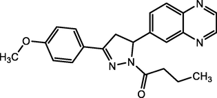
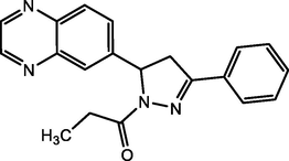
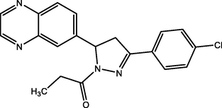
1.
1-[3-(4-methylphenyl)-5-(quinoxalin-6-yl)-4,5-dihydropyrazol-1-yl]butan-1-one
(Me-4-PQPB)

80.42
Olasunkanmi et al. (2016a)
2.
1-[3-(4-methoxyphenyl)-5-(quinoxalin-6-yl)-4,5-dihydro-1H-pyrazol-1-yl]butan-1-one
(Mt-4-PQPB)
72.01
Olasunkanmi et al. (2016a)
3.
1-[3-(3-methoxylphenyl)-5-(quinoxalin-6-yl)-4,5-dihydropyrazol-1-yl]butan-1-one
(Mt-3-PQPB)
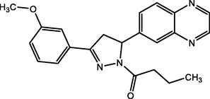
69.66
Olasunkanmi et al. (2016a)
4.
1-[3-(2H-1,3-benzodioxol-5-yl)-5-(quinoxalin-6-yl)-4,5-dihydropyrazol-1-yl]butan-1-one
(Oxo-PQPB)
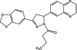
68.41
Olasunkanmi et al. (2016a)
5.
1-[3-(phenyl-5-quinoxalin-6-yl)-4,5-dihydro-1H-pyrazol-1-yl]butan-1-one
(PQDPB)
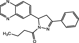
90.50
Olasunkanmi et al. (2015)
6.
1-[3-(phenyl-5-quinoxalin-6-yl)-4,5-dihydro-1H-pyrazol-1-yl]propan-1-one
(PQDPP)
93.65
Olasunkanmi et al. (2015)
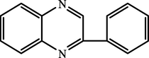
7.
2-phenyl-1-[3-phenyl-5-(quinoxalin-6-yl)-4,5-dihydro-1H-pyrazol-1-yl]ethanone
(PPQDPE)
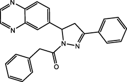
86.88
Olasunkanmi et al. (2015)
8.
N-{2-[1-propanoyl-5-(quinoxalin-6-yl)-4,5-dihydro-1H-pyrazol-3-yl]phenyl}methanesulfonamide
(MS-2-PQPP)
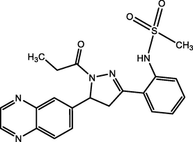
91.54
Olasunkanmi et al. (2016b)
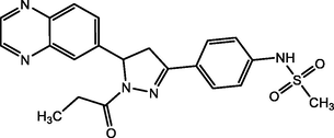
9.
N-{3-[1-propanoyl-5-(quinoxalin-6-yl)-4,5-dihydro-1H-pyrazol-3-yl]phenyl}methanesulfonamide
(MS-3-PQPP)
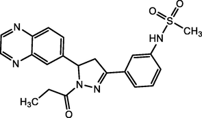
93.88
Olasunkanmi et al. (2016b)
10.
N-{4-[1-propanoyl-5-(quinoxalin-6-yl)-4,5-dihydropyrazol-3-yl]phenyl}methanesulfonamide
(MS-4-PQPP)
93.56
Olasunkanmi et al. (2016b)
11.
N-{2-[1-(methanesulfonyl)-5-(quinoxalin-6-yl)-4,5-dihydro-1H-pyrazol-3-yl]phenyl}methanesulfonamide
(MS-2-PQPMS)

92.68
Olasunkanmi et al. (2016b)
12.
N-{3-[1-(methanesulfonyl)-5-(quinoxalin-6-yl)-4,5-dihydro-1H-pyrazol-3-yl]phenyl}methanesulfonamide
(MS-3-PQPMS)
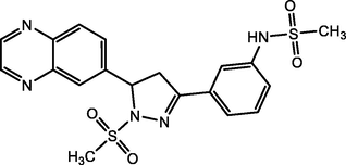
93.39
Olasunkanmi et al. (2016b)
13.
N-{4-[1-(methanesulfonyl)-5-(quinoxalin-6-yl)-4,5-dihydro-1H-pyrazol-3-yl]phenyl}methanesulfonamide
(MS-4-PQPMS)
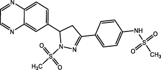
94.00
Olasunkanmi et al. (2016b)
14.
1-[3-(3-methoxyphenyl)-5-(quinoxalin-6-yl)-4,5-dihydropyrazol-1-yl]propan-1-one
(Mt-3-PQPP)
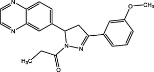
93.69
Olasunkanmi and Ebenso (2020)
15.
1-(3-(4-chlorophenyl)-5-(quinoxalin-6-yl)-4,5-dihydro-1H-pyrazol-1-yl)propan-1-one
(Cl-4-PQPP)
92.27
Olasunkanmi and Ebenso (2020)
16.
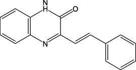
(E)-1-benzyl-3-(4-methoxystyryl)quinoxalin-2(1H)-one
(QN1)
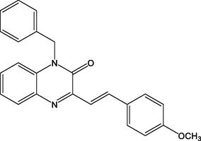
93.00
Lgaz et al. (2016a)
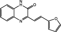
17.
(E)-3-(2-(furan-2-yl)vinyl)quinoxalin-2(1H)-one
(QN2)
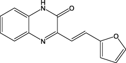
90.00
Lgaz et al. (2016a)
18.
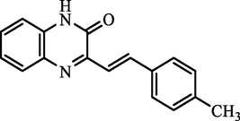
(E)-3-(4-methoxystyryl)quinoxalin-2(1H)-one
(QN3)
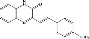
87.00
Lgaz et al. (2016a)
19.
(E)-3-styrylquinoxalin-2(1H)-one
(QN4)
85.00
Lgaz et al. (2016a)
20.
3-methyl-1-prop-2-ynylquinoxalin-2(1H)-one
(Pr-N-Q = O)
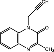
88.80
El-Hajjaji et al. (2014)
21.
3-methyl-1-prop-2-ynylquinoxaline-2(1H)-thione
(Pr-N-Q = S)

92.30
El-Hajjaji et al. (2014)
22.
Quinoxaline
(QX)
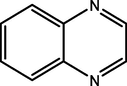
84.20
Fu et al. (2012)
23.
2-chloroquinoxaline
(CHQX)
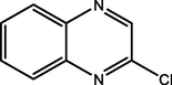
92.50
Fu et al. (2012)
24.
2-quinoxalinethiol
(THQX)
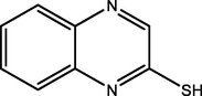
95.50
Fu et al. (2012)
25.
4-(quinoxalin-2-yl)phenol
(PHQX)
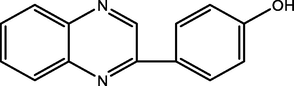
98.30
Fu et al. (2012)
26.
3-methylquinoxalin-2(1H)-one
(Q = O)
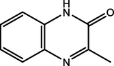
66.60
Benbouya et al. (2012)
27.
3-methylquinoxalin-2(1H)-thione
(Q = S)
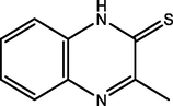
82.80
Benbouya et al. (2012)
28.
7-chloro-3-methylquinoxalin-2(1H)-thione
(Cl-Q = S)
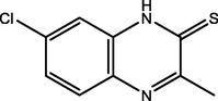
75.00
Benbouya et al. (2012)
29.
7-chloro-2-(4-methoxyphenyl)thieno[2,3-b]quinoxaline
(CMOPTQ)
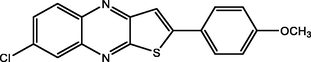
89.00
Adardour et al. (2013)
30.
7-chloro-3-(4-methoxystyryl)quinoxalin-2-one
(CMOSQ)
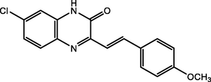
87.00
Adardour et al. (2013)
31.
(E)-3-(4-methoxystyryl)-7-methylquinoxalin-2(1H)-one
(MOSMQ)
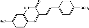
92.00
Tazouti et al. (2016)
32.
(E)-3-(2-(furan-2-yl)vinyl) quinoxalin2(1H)-one
(FVQ)
94.98
Lgaz et al. (2016b)
33.
3,7-dimethylquinoxalin-2 (1H)-one
(DMQ = O)
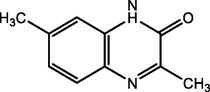
88.07
Adardour et al. (2010)
34.
3,7-dimethylquinoxalin-2 (1H)-thione
(DMQ = S)
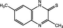
93.27
Adardour et al. (2010)
35.
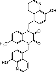
1,4-bis((8-hydroxyquinolin-5-yl)-methyl)-6-methylquinoxalin-2,3-(1H,4H)-dione
(Q-HNHyQ)
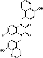
89.40
Rbaa et al. (2018)
36.
1,4-bis-((8-hydroxyquinolin-5-yl)-methyl)-quinoxalin-2,3-(1H,4H)-dione (QCH3NHyQ)
95.40
Rbaa et al. (2018)
37.
2-(2,4-dichlorophenyl)-1,4-dihydroquinoxaline
(HQ)
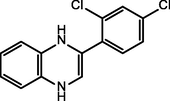
91.00
Benhiba et al., 2020
38.
2-(2,4-dichlorophenyl)-6-methyl-1,4-dihydroquinoxaline
(CQ)
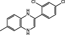
94.20
Benhiba et al., 2020
39.
(E)-3-(4-chlorostyryl)quinoxalin-2(1H)-one
(CSQN)
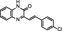
92.80
Laabaissi et al. (2020)
40.
(E)-3-(4-(dimethylamino)styryl)quinoxalin-2(1H)-one
(NSQN)
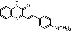
96.40
Laabaissi et al. (2020)
2.2 Molecular descriptors calculation
The study considered molecular descriptors derived from quantum chemical calculations and Dragon 7 software. Quantum chemical descriptors were generated by carrying out DFT calculations using B3LYP functional with 6-31+(d,p) basis set on the neutral forms of the quinoxaline molecules in aqueous and gaseous phases.The chemical structures of the quinoxalines were modelled using ChemDraw Professional 15.0 software and viewed using Gaussview 5.0. Optimizations of the molecules to a local minimum were performed using Gaussian 09 software and full optimization was verified by the absence of imaginary vibrational frequencies. Total energy (TE), dipole moment (μ) and energies of the lowest unoccupied molecular orbital (ELUMO) and highest occupied molecular orbital (EHOMO) were obtained for all the studied molecules. Other molecular descriptors for the inhibitor molecules were calculated using the following equations (Yusuf et al., 2020, Quadri et al., 2021a).
Using the optimized molecular structures, numerous molecular descriptors were obtained from Dragon 7 (Mauri et al., 2006). Dragon 7 is a software application that calculates above 5000 molecular descriptors (0D, 1D, 2D and 3D) divided into 30 categories which can be used for QSPR modelling. Optimized quinoxaline molecules were converted from .log to .mdl file format using Open Babel (O'Boyle et al., 2011) and were used as inputs into Dragon 7 to calculate a host of molecular descriptors. Preliminary eliminations of high dimensional descriptors were done using the Dragon 7 software to remove descriptors with missing entries, descriptors with zero values and those with constant and/or near constant values. In addition, multicollinear descriptors and descriptors having standard deviation (SD) lower than 0.0001 were removed. The filtered descriptors were combined with DFT-based descriptors and subjected to standardization with the aim of ranking the descriptors in order of relative significance to the experimental IE%. This process was performed using Minitab 7.
2.3 Statistical modelling
Ordinary least squares regression, a form of MLR, was utilized to model the linear correlation between the filtered chemical variables (X) and the inhibition performance (Y) where X denotes the independent variable and Y is the dependent variable. The OLS regression was carried out using Minitab 7 and characterized by correlation coefficient and standard deviation.
On the other hand, ANN was adopted to model the nonlinear relationship between the chosen chemical variables and the inhibition performances of the investigated 40 quinoxaline molecules. Using a supervised learning method and a feedforward backpropagation architecture, neural network modelling was performed using Matlab. Six input parameters comprising five selected constitutional indices and inhibitor concentration served as the inputs, while three hidden neurons governed by logsig activation function and five hidden neurons controlled by the softmax activation function were utilized to model the output inhibition efficiencies (Fig. 1). The Levenberg-Marquardt training algorithm was implemented because of its effectiveness and quick convergence. Several iterations (training and retraining) were carried out until a low statistical error value was obtained.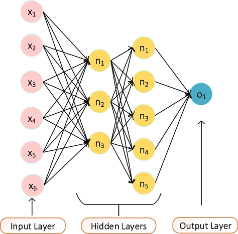
ANN architecture for the model.
2.4 Statistical criteria
The performance of the linear model was characterized using R2 and SD while the nonlinear model was characterized using several statistical criteria. Statistically robust and reliable models are demonstrated by low statistical error values. The main statistical parameters are obtained using the following relationships (Gramatica 2013, Eftekhari et al., 2018, Liu et al., 2019, Olatunji et al., 2019, Adedeji et al., 2020a,b):
Root mean square error,
Mean square error,
Mean average deviation,
Mean average percentage error,
Coefficient of variation,
Relative mean bias error,
3 Results and discussion
3.1 DFT studies of selected quinoxalines
Inhibition performances of organic corrosion inhibitors of metal are closely correlated with their chemical stability or reactivity. The chemical reactivity of a series of chemical compounds are predicted by the analysis of frontier molecular orbital (FMO) theory. The theory gives useful insight on the probable adsorption centres of the organic molecules under study. From the presented images in Table 2, it is clear that the LUMO and HOMO energy orbitals in aqueous phase are widely spread on the quinoxaline moiety with minimal extension to the different substituent groups in some cases. This indicates that these sites would be the sites of preference for adsorption onto the mild steel (Fu et al., 2012, Olasunkanmi and Ebenso 2020). It should also be noted that there are a few cases where the HOMO and LUMO are localized around the phenyl rings (MS-n-PQPP series) (Olasunkanmi et al., 2016) and a few other cases where nearly all the atoms in the quinoxaline molecule act as sites of adsorption.
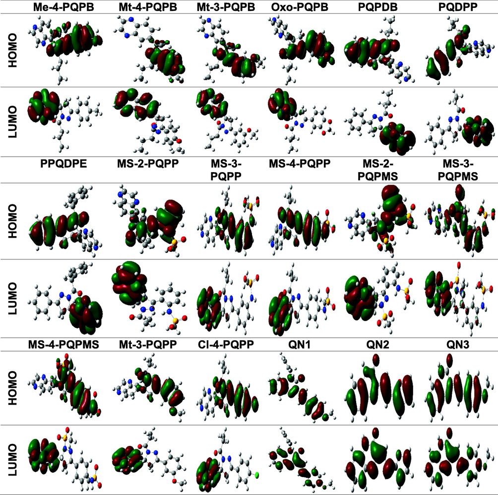
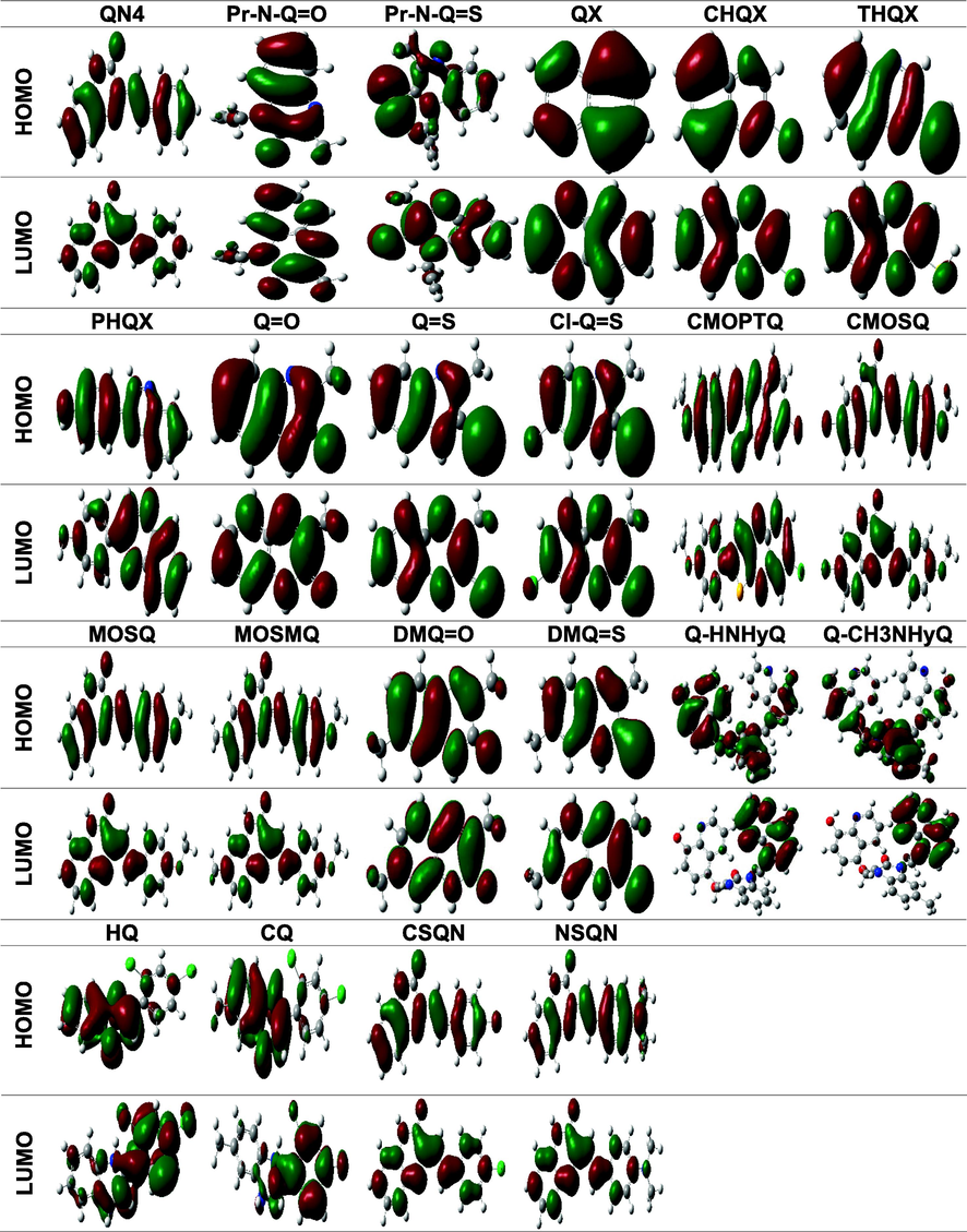
Generally, the adherence capacity of inhibitor compounds can be explained as a donor–acceptor interface between the investigated compounds and the metal of interest. EHOMO is proportional to the electron contributing potential of the studied inhibitor, while ELUMO is connected to the electron accepting potential of the investigated compound. Lesser values of energy gap, ΔE are reported to imply higher inhibition efficiencies as these molecules undergo ease of transfer of one or more electrons from the HOMO level to the metallic orbital (Olasunkanmi et al., 2015, Benhiba et al., 2020). Studies have also shown that a hard molecule possesses higher values of energy gap, while the reverse occurs for soft molecules. It is therefore expected that a compound with a greater value of softness and lesser value of hardness will be more reactive and consequently favour adsorption potential ((Lgaz et al., 2016a) (Olasunkanmi et al., 2016a)). Lower TE also indicates that the quinoxaline compound adsorbs favourably through the active adsorption sites (Benhiba et al., 2020). The calculated DFT variables shown in Table 3 for the investigated quinoxalines do not follow any particular trend with respect to the reported experimental IE% due to the complex nature of the reaction occurring at the mild steel/electrolyte interface. The factors affecting the IE% of the quinoxaline-based inhibitors are quite numerous (Li et al., 2015).
Quinoxalines
Conc* (M)
Temp* (K)
Phase
TE
(eV)EHOMO (eV)
ELUMO (eV)
ΔΕ (eV)
µ
(D)IP
(eV)EA
(eV)Χ
(eV)η
(eV)σ
(eV−1)ΔΝ
IE%*
Me-4-PQPB
0.000280
303
G
−31182.23
−6.035
−2.269
3.766
4.738
6.035
2.269
4.152
1.883
0.531
0.756
80.42
A
−31182.71
−6.143
−2.418
3.725
7.156
6.143
2.418
4.281
1.863
0.537
0.730
Mt-4-PQPB
0.000270
303
G
−33228.80
−5.839
−2.249
3.590
5.114
5.839
2.249
4.044
1.795
0.557
0.823
72.01
A
−32610.20
−6.160
4.946
11.106
2.632
6.160
−4.946
0.607
5.553
0.180
0.576
Mt-3-PQPB
0.000270
303
G
−33228.78
−6.077
−2.258
3.819
5.462
6.077
2.258
4.168
1.909
0.524
0.742
69.66
A
−32610.18
−6.523
4.949
11.471
3.332
6.523
−4.949
0.787
5.736
0.174
0.542
Oxo-PQPB
0.000260
303
G
−34588.63
−6.211
4.910
11.121
2.353
6.211
−4.910
0.650
5.561
0.180
0.571
68.41
A
−35243.16
−5.912
−2.417
3.495
7.146
5.912
2.417
4.165
1.747
0.572
0.811
PQPDB
0.000170
303
G
−29550.99
−6.574
4.927
11.502
2.529
6.574
−4.927
0.824
5.751
0.174
0.537
90.50
A
−30112.69
−6.256
−2.421
3.835
6.313
6.256
2.421
4.338
1.918
0.521
0.694
PQDPP
0.000180
303
G
−28501.14
−6.580
4.925
11.505
2.546
6.580
−4.925
0.827
5.753
0.174
0.537
93.65
A
−28501.14
−6.580
4.925
11.505
2.547
6.580
−4.925
0.827
5.753
0.174
0.537
PPQDPE
0.000150
303
G
−34260.11
−6.202
−2.270
3.932
4.117
6.202
2.270
4.236
1.966
0.509
0.703
86.88
A
−34260.62
−6.296
−2.422
3.874
6.546
6.296
2.422
4.359
1.937
0.516
0.682
MS-2-PQPP
0.000240
303
G
−46546.65
−6.327
−2.403
3.925
6.173
6.327
2.403
4.365
1.962
0.510
0.671
91.54
A
−46547.39
−6.325
−2.437
3.888
9.869
6.325
2.437
4.381
1.944
0.514
0.674
MS-3-PQPP
0.000240
303
G
−45739.13
−6.739
4.869
11.608
5.577
6.739
−4.869
0.935
5.804
0.172
0.522
93.88
A
−31560.33
−6.527
4.947
11.474
3.342
6.527
−4.947
0.790
5.737
0.174
0.541
MS-4-PQPP
0.000240
303
G
−45739.16
−6.470
4.844
11.314
4.062
6.470
−4.844
0.813
5.657
0.177
0.547
93.56
A
−46547.38
−6.118
−2.422
3.695
7.497
6.118
2.422
4.270
1.848
0.541
0.739
MS-2-PQPMS
0.000230
303
G
−57319.91
−6.589
−2.420
4.169
9.081
6.589
2.420
4.505
2.085
0.480
0.598
92.68
A
−57320.90
−6.471
−2.448
4.023
14.915
6.471
2.448
4.460
2.012
0.497
0.631
MS-3-PQPMS
0.000230
303
G
−56372.15
−7.070
4.861
11.931
4.737
7.070
−4.861
1.105
5.966
0.168
0.494
93.39
A
−45739.13
−6.739
4.869
11.608
5.577
6.739
−4.869
0.935
5.804
0.172
0.522
MS-4-PQPMS
0.000230
303
G
−57319.87
−6.369
−2.369
4.000
5.952
6.369
2.369
4.369
2.000
0.500
0.658
94.00
A
−57320.89
−6.373
−2.441
3.932
11.481
6.373
2.441
4.407
1.966
0.509
0.659
Mt-3-PQPP
0.000275
303
G
−31560.33
−6.527
4.947
11.474
3.342
6.527
−4.947
0.790
5.737
0.174
0.541
93.69
A
−31560.33
−6.527
4.947
11.474
3.342
6.527
−4.947
0.790
5.737
0.174
0.541
Cl-4-PQPP
0.000275
303
G
−40855.49
−6.823
4.834
11.658
1.247
6.823
−4.834
0.995
5.829
0.172
0.515
92.27
A
−40855.49
−6.823
4.834
11.658
1.247
6.823
−4.834
0.995
5.829
0.172
0.515
QN1
0.005000
303
G
−32290.52
−5.591
−2.421
3.170
0.539
5.591
2.421
4.006
1.585
0.631
0.945
93.00
A
−31687.93
−5.667
4.602
10.269
1.860
5.667
−4.602
0.533
5.135
0.195
0.630
QN2
0.005000
303
G
−21756.03
−5.742
−2.606
3.136
2.513
5.742
2.606
4.174
1.568
0.638
0.901
90.00
A
−21756.41
−5.845
−2.739
3.106
3.753
5.845
2.739
4.292
1.553
0.644
0.872
QN3
0.005000
303
G
−24467.82
−5.714
4.585
10.299
1.733
5.714
−4.585
0.564
5.149
0.194
0.625
87.00
A
−24467.82
−5.713
4.584
10.297
1.733
5.713
−4.584
0.565
5.149
0.194
0.625
QN4
0.005000
303
G
−21408.61
−5.959
4.529
10.488
2.008
5.959
−4.529
0.715
5.244
0.191
0.599
85.00
A
−21408.61
−5.959
4.530
10.489
2.008
5.959
−4.530
0.715
5.244
0.191
0.599
Pr-N-Q = O
0.001000
303
G
−17304.46
−6.355
5.263
11.618
2.056
6.355
−5.263
0.546
5.809
0.172
0.555
88.80
A
−17634.00
−6.593
−2.226
4.367
4.608
6.593
2.226
4.410
2.184
0.458
0.593
Pr-N-Q = S
0.001000
303
G
−26421.81
−6.044
−2.555
3.488
4.015
6.044
2.555
4.299
1.744
0.573
0.774
92.30
A
−26422.09
−6.292
−2.680
3.612
6.436
6.292
2.680
4.486
1.806
0.554
0.696
QX
0.001000
298
G
−11374.34
−6.987
−2.299
4.688
0.596
6.987
2.299
4.643
2.344
0.427
0.503
84.20
A
−11374.52
−7.031
−2.382
4.649
0.765
7.031
2.382
4.706
2.325
0.430
0.493
CHQX
0.001000
298
G
−23880.88
−7.184
−2.533
4.651
2.399
7.184
2.533
4.859
2.325
0.430
0.460
92.50
A
−23881.05
−7.144
−2.554
4.590
3.161
7.144
2.554
4.849
2.295
0.436
0.469
THQX
0.001000
298
G
−22209.92
−6.620
−2.326
4.295
1.087
6.620
2.326
4.473
2.147
0.466
0.588
95.50
A
−22210.15
−6.659
−2.386
4.273
1.422
6.659
2.386
4.522
2.136
0.468
0.580
PHQX
0.001000
298
G
−19709.40
−6.187
−2.240
3.947
1.951
6.187
2.240
4.214
1.974
0.507
0.706
98.30
A
−19709.72
−6.263
−2.386
3.877
2.435
6.263
2.386
4.325
1.938
0.516
0.690
Q = O
0.001000
308
G
−14492.12
−6.538
−2.117
4.421
3.335
6.538
2.117
4.328
2.210
0.452
0.604
66.60
A
−14492.44
−6.553
−2.168
4.384
4.846
6.553
2.168
4.360
2.192
0.456
0.602
Q = S
0.001000
308
G
−23280.35
−6.115
−2.573
3.541
4.192
6.115
2.573
4.344
1.771
0.565
0.750
82.80
A
−23280.66
−6.271
−2.649
3.622
6.751
6.271
2.649
4.460
1.811
0.552
0.701
Cl-Q = S
0.001000
308
G
−35786.78
−6.275
−2.759
3.516
2.501
6.275
2.759
4.517
1.758
0.569
0.706
75.00
A
−35787.08
−6.355
−2.747
3.609
4.469
6.355
2.747
4.551
1.804
0.554
0.679
CMOPTQ
0.010000
303
G
−45481.52
−6.199
4.034
10.233
4.906
6.199
−4.034
1.082
5.116
0.195
0.578
89.00
A
−45481.52
−6.199
4.034
10.233
4.906
6.199
−4.034
1.082
5.116
0.195
0.578
CMOSQ
0.010000
303
G
−36822.14
−5.919
4.236
10.156
1.767
5.919
−4.236
0.842
5.078
0.197
0.606
87.00
A
−37439.97
−5.805
−2.731
3.074
1.689
5.805
2.731
4.268
1.537
0.651
0.889
MOSMQ
0.000100
298
G
−25517.79
−5.633
4.640
10.274
2.138
5.633
−4.640
0.496
5.137
0.195
0.633
92.00
A
−25517.79
−5.633
4.640
10.274
2.138
5.633
−4.640
0.496
5.137
0.195
0.633
FVQ
0.000100
298
G
−21756.03
−5.742
−2.606
3.136
2.513
5.742
2.606
4.174
1.568
0.638
0.901
94.00
A
−21756.41
−5.845
−2.739
3.106
3.753
5.845
2.739
4.292
1.553
0.644
0.872
DMQ = O
0.000100
298
G
−15271.34
−6.267
5.384
11.651
2.631
6.267
−5.384
0.441
5.825
0.172
0.563
88.07
A
−15271.34
−6.267
5.384
11.651
2.631
6.267
−5.384
0.441
5.825
0.172
0.563
DMQ = S
0.010000
298
G
−23960.66
−5.348
4.890
10.239
2.871
5.348
−4.890
0.229
5.119
0.195
0.661
93.27
A
−23960.66
−5.348
4.890
10.238
2.871
5.348
−4.890
0.229
5.119
0.195
0.661
Q-HNHyQ
0.001000
298
G
−42704.01
−6.235
5.150
11.384
3.496
6.235
−5.150
0.542
5.692
0.176
0.567
89.40
A
−42704.01
−6.235
5.150
11.384
3.496
6.235
−5.150
0.542
5.692
0.176
0.567
Q-CH3NHyQ
0.001000
298
G
−44583.73
−6.081
−2.033
4.047
6.401
6.081
2.033
4.057
2.024
0.494
0.727
95.40
A
−43753.97
−6.172
5.158
11.329
3.774
6.172
−5.158
0.507
5.665
0.177
0.573
HQ
0.001000
303
G
−42072.41
−5.323
5.519
10.842
1.961
5.323
−5.519
−0.098
5.421
0.184
0.655
91.00
A
−42707.73
−4.741
−1.263
3.478
2.418
4.741
1.263
3.002
1.739
0.575
1.149
CQ
0.001000
303
G
−43777.44
−4.566
−1.266
3.300
2.024
4.566
1.266
2.916
1.650
0.606
1.238
94.20
A
−43122.36
−5.251
5.541
10.793
2.131
5.251
−5.541
−0.145
5.396
0.185
0.662
CSQN
0.001000
303
G
−33762.98
−6.162
4.271
10.433
4.983
6.162
−4.271
0.946
5.217
0.192
0.580
92.80
A
−33762.98
−6.162
4.271
10.433
4.984
6.162
−4.271
0.946
5.217
0.192
0.580
NSQN
0.001000
303
G
−24986.21
−5.445
4.659
10.104
1.236
5.445
−4.659
0.393
5.052
0.198
0.654
96.40
A
−24986.21
−5.445
4.659
10.104
1.236
5.445
−4.659
0.393
5.052
0.198
0.654
3.2 Feature selection
Few highly informative descriptors from the numerous calculated quantum chemical and Dragon-based descriptors were obtained using feature selection. The MLR standardization method was adopted to carry out feature selection by ranking all the obtained molecular descriptors in order of their standardized coefficients or relative significance. Fig. 2 shows the significant features among the numerous molecular descriptors. The five topmost descriptors shown in Fig. 2 were utilized along with concentration in QSPR analysis using linear modelling (MLR) and nonlinear modelling (ANN) techniques. The selected descriptors (MW, nCsp2, nCsp3, nO and nN) have been described in Table 4. In addition, the plot of the Pearson’s correlation matrix of the selected chemical variables is presented in Table 5.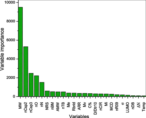
Significance of molecular descriptors to the inhibition efficiencies of quinoxalines.
Descriptors
Group name
Description
MW
Constitutional indices
Molecular weight
nN
Constitutional indices
Number of nitrogen atoms
nO
Constitutional indices
Number of oxygen atoms
nCsp3
Constitutional indices
Number of sp3 hybridized carbon atoms
nCsp2
Constitutional indices
Number of sp2 hybridized carbon atoms
Conc
MW
nN
nO
nCsp3
nCsp2
IE%
Conc
1
−0.224
−0.473
−0.123
−0.427
−0.018
0.103
MW
−0.224
1
0.845
0.819
0.697
0.818
0.108
nN
−0.473
0.845
1
0.709
0.849
0.482
0.023
nO
−0.123
0.819
0.709
1
0.504
0.629
0.079
nCsp3
−0.427
0.697
0.849
0.504
1
0.341
−0.246
nCsp2
−0.018
0.818
0.482
0.629
0.341
1
0.165
IE%
0.103
0.108
0.023
0.079
−0.246
0.165
1
3.3 MLR model
The obtained mathematical relation representing the QSPR model of investigated quinoxalines using the OLS method is as follows:
R2 = 0.3009, SD = 7.24607 where MW, nN, nO, nCsp2 and nCsp3 are the screened descriptors of interest and Conc denotes the concentration of quinoxalines. The developed OLS model clearly showed that the IE% of studied quinoxalines are influenced by increase in Conc, MW, nN and decrease in nO, nCsp3 and nCsp2. The screened descriptors are constitutional indices, which are known to affect the adherence ability of quinoxalines on mild steel surface. Numerous corrosion scientists have investigated the adsorption ability of organic molecules such as quinoxalines with oxygen and nitrogen atoms. These heteroatoms serve as active sites of adsorption thereby offering effective protection for the metal from corrosive ions. In addition, molecules having high molecular weight and sp2 and sp3 hybridized carbon atoms have been established to be effective corrosion inhibitors as they serve as anchoring sites for molecular adherence on the metallic substrate ((Lgaz et al., 2016a; Olasunkanmi et al., 2016a) Benhiba et al., 2020, Olasunkanmi and Ebenso, 2020).
Table 6 presents the ANOVA and regression coefficients table, which shows a p-value slightly higher than expected. It is clear that the model lacks the capability to accurately explain the inhibition mechanism of quinoxalines on the account of its low R2, high SD and high sum of squares error (SSE). Thus, it is mandatory to employ a nonlinear model to further investigate the relationship between the screened variables and the IE% of quinoxaline-based corrosion inhibitors.
Source
DF
Adj SS
Adj MS
F-value
p-value
Regression
6
745.92
124.320
2.37
0.052
Conc
1
15.58
15.578
0.30
0.590
MW
1
37.94
37.942
0.72
0.401
nN
1
127.18
127.180
2.42
0.129
nO
1
67.97
67.969
1.29
0.263
nCsp3
1
649.92
649.924
12.38
0.001
nCsp2
1
4.06
4.056
0.08
0.783
Error
33
1732.68
52.506
Lack-of-Fit
28
1725.83
61.637
44.97
0.000
Pure Error
5
6.85
1.371
Total
39
2478.60
Term
Coeff
SE Coeff
T-value
p-value
Constant
74.84
5.860
12.77
0.000
Conc
270.00
496.000
0.54
0.590
MW
0.04
0.052
0.85
0.401
nN
4.92
3.160
1.56
0.129
nO
−1.89
1.660
−1.14
0.263
nCsp3
−4.00
1.140
−3.52
0.001
nCsp2
−0.17
0.613
−0.28
0.783
3.4 ANN model: internal validation
The inadequacy of the proposed linear model mandated the development of a nonlinear model to better comprehend the relationship between the descriptors and the IE% for quinoxaline compounds studied as anticorrosive agents. The neural network models were established to model the connection between the experimental IE% and the predicted IE%. The internal validation was carried out using k-fold validation technique. A k-fold of 5 was used which implies that the quinoxaline dataset was randomly divided into five equal groups and four groups (i.e., 32 compounds) were used to train the model in each case and one group (i.e., 8 compounds) was utilized to check the accuracy of the established model.
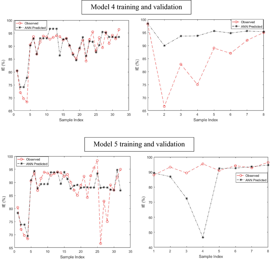
The results of the training and validation phase of the ANN built models for quinoxaline inhibitors are displayed in Fig. 3. The plots show instances of the calculated IE% diverging from the measured IE%. These divergences are observed both at the training and validation phases of the model development process. At the training phase, models 1 and 2 showed clear cases of underprediction while model 5 was clearly overpredicting the measured IE%. Models 3 and 4 revealed fair cases of divergence. At the validation stage, models 2, 4 and 5 clearly underpredict the checking dataset, while model 3 is a case of overprediction. These observed discrepancies between the experimental and calculated IE% are attributed to the misfiring of the neural network node (Adedeji et al., 2019).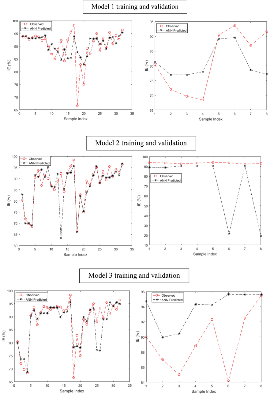
Experimental IE% and predicted IE% at the model training and validation phase for quinoxaline derivatives (models 1–5).
Experimental IE% and predicted IE% at the model training and validation phase for quinoxaline derivatives (models 1–5).
ANN architecture used for model development was reported on Table 7 as 6-3-5-1. This implies that six molecular variables were used as input variables with 3 and 5 neurons at the hidden layers and an output of IE%. The error estimates between the measured and the predicted IE% have been established to be a reliable means of assessing the ability of the proposed models. Several statistical performance indices have been employed in this work to appraise the reliability and predictive power of the developed models. These include error functions such as MSE, RMSE, MAD and MAPE. These have been reported in other fields as excellent metrics to evaluate neural network models (Aouidate et al., 2016, Abdel-Ilah et al., 2017, Eftekhari et al., 2018). The selection of the best model is achieved by considering the model that yields the lowest values of these error functions and also shows minor variance between the training and validation phase (Gramatica, 2013). On this basis, the five proposed models with their respective error functions have been displayed in Table 7.
Metric
Model 1
Model 2
Model 3
Model 4
Model 5
Average
Train
Validation
Train
Validation
Train
Validation
Train
Validation
Train
Validation
Train
Validation
MSE
27.7813
57.9311
32.1215
1304.0
21.2783
29.3336
8.9254
140.9121
30.7511
338.9934
24.1715
380.4940
RMSE
5.2708
7.6112
5.6676
36.5421
4.6128
5.4160
2.9875
11.8706
5.5454
18.4118
4.8168
15.9703
MAD
3.3810
6.3525
2.7213
26.0772
2.8527
2.3816
2.0521
6.5330
3.6843
11.9122
2.9383
10.6513
MAPE
4.0055
7.9444
2.8803
22.1418
3.3460
5.0389
2.3188
11.7086
4.4810
10.5053
3.4063
11.4678
rMBE
0.5134
−0.8351
−1.1694
−22.1535
−0.8127
4.9120
0.6472
10.3818
0.3852
−9.7155
−2.1074
−3.4821
CoV
0.0171
0.0174
0.0440
0.0091
0.0296
0.0112
0.27
0.0098
0.0138
0.0357
0.1503
0.0166
Iterations
141
245
64
620
471
–
Topology
6-3-5-1
6-3-5-1
6-3-5-1
6-3-5-1
6-3-5-1
6-3-5-1
A careful comparison of the presented data in the table shows that model 3 could be adjudged to be the least biased to the selected dataset, based on statistical error analyses tools. This is because model 3 is characterized by consistent lower values of MSE, RMSE, MAD and MAPE when compared to the other developed models. Models 1 and 4 showed some promising error functions at some levels but were inconsistent with large variance between the training and validation phase.
3.5 ANN model: external validation
From the above findings and using the variants of molecules that yielded the highest inhibition efficiencies from experimental assessments, ten new quinoxaline compounds were theoretically designed. The inhibition performances of these novel quinoxalines were assessed using the QSPR models developed from MLR and ANN techniques. The calculated descriptors of the novel quinoxalines obtained from Dragon 7.0 software are displayed in Table 8.
Compounds
Conc
MW
nN
nO
nCsp3
nCsp2
A
0.001
256.32
2
0
0
18
B
0.001
206.26
2
0
0
14
C
0.001
222.26
2
1
0
14
D
0.001
220.29
2
0
1
14
E
0.001
251.26
3
2
0
14
F
0.001
264.30
2
2
0
16
G
0.001
262.33
2
1
1
16
H
0.001
293.30
3
3
0
16
I
0.001
282.74
2
1
0
16
J
0.001
286.35
2
1
1
18
The chemical names and structures of the novel quinoxalines proposed as efficient anticorrosive agents for mild steel deterioration in HCl at 0.001 M are presented on Table 9. The predicted inhibition performances ranged from 87.88 to 94.77% for MLR model and 94.59 to 95.73% for the ANN model. The predicted IE% from the developed MLR and ANN models show that the novel quinoxalines are excellent inhibitors of acidic corrosion. The effect of the presence of substituents on the IE% of the newly designed quinoxaline molecules are also observed as is often reported in literature (Fu et al., 2012, Lgaz et al., 2016b, Tazouti et al., 2016, Benhiba et al., 2020).
Quinoxalines
IUPAC nomenclature
Molecular structure
MLR predicted IE%
ANN predicted IE%
A.
2-phenylquinoxaline
93.17
94.80
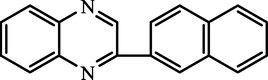
B.
2-(naphthalen-2-yl)quinoxaline
91.65
95.65
C.
3-(quinoxalin-2-yl)phenol
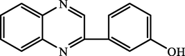
90.46
95.60
D.
2-(p-tolyl)quinoxaline
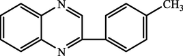
88.26
95.21
E.
2-(4-nitrophenyl)quinoxaline

94.77
95.73
F.
(E)-3-(4-hydroxystyryl)quinoxalin-2(1H)-one
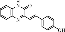
90.08
95.60
G.
(E)-3-(4-methylstyryl)quinoxalin-2(1H)-one
87.88
95.27
H.
(E)-3-(4-nitrostyryl)quinoxalin-2(1H)-one
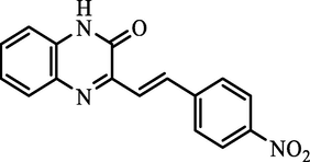
94.39
95.66
I.
(E)-7-chloro-3-styrylquinoxalin-2(1H)-one
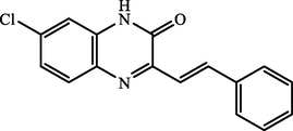
92.78
95.46
J.
(E)-3-(2-(1H-inden-7-yl)vinyl)quinoxalin-2(1H)-one
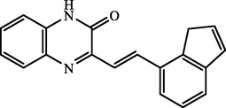
88.60
94.59
Fig. 4 showed a graphical representation of the predicted IE% from MLR and ANN models. It is obvious from the plot that the best ANN model showed a better surface coverage of the novel quinoxaline-based inhibitors on the mild steel surface in molar HCl than the linear model.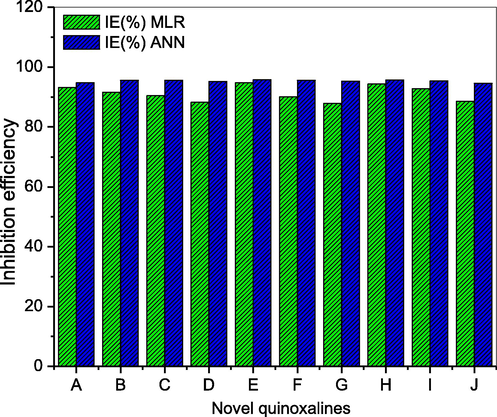
Comparison of predicted IE% of novel quinoxalines obtained with MLR and ANN models.
A statistical analysis to ascertain whether the difference between the MLR and ANN models for the inhibition performance of the novel quinoxalines is statistically significant was conducted and the outcome is presented in Table 10. At a confidence level of 0.05, F (26.31093) > Fcrit (4.413873) which shows that there is a statistically significant variance between the MLR and ANN models for the test dataset.
Source of variation
SS
df
MS
F
p-value
Fcrit
Between Groups
86.22407
1
86.22407
26.31093
7.02E-05
4.413873
Within Groups
58.98817
18
3.27712
Total
145.2122
19
4 Conclusions
-
Quantum chemical studies of 40 quinoxalines was performed and the orbital density distribution images provided information on the probable sites of adsorption. Molecular descriptors were calculated using DFT method and Dragon 7 software.
-
Linear model showed poor correlation with the experimental IE% and high statistical error values which portends that corrosion inhibition mechanism is a complex nonlinear process that is affected by many factors. Nonlinear neural network presented a more reliable and robust alternative to modelling inhibition data to gain insight into inhibition mechanism.
-
The established models suggest that the considered constitutional indices comprising molecular weight, number of oxygen atoms, number of nitrogen atoms and number of hybridized carbon atoms form an efficient group of molecular descriptors for QSPR modelling of quinoxaline inhibitors. Thus, constitutional indices are crucial for determining the inhibition efficiencies of quinoxaline molecules.
-
Excellent inhibition performances of the 10 novel quinoxaline-based inhibitors obtained from the forecast using the developed QSPR models suggest that the non-synthesized compounds are potential organic compounds that can be explored experimentally as safe and effective inhibitors of metallic deterioration in molar HCl.
CRediT authorship contribution statement
Taiwo W. Quadri: Investigation, Data curation, Writing-Original draft. Lukman O. Olasunkanmi: Investigation, Data curation, Writing-Original draft. Omolola E. Fayemi: Investigation, Data curation, Writing-Original draft. Hassane Lgaz: Methodology, Validation, Formal analysis, Writing - Review & Editing, Supervision, Funding acquisition. Omar Dagdag: Investigation, Data Curation, Software, Writing - Review & Editing. El-Sayed M. Sherif: Investigation, Data Curation, Software, Writing - Review & Editing. Awad A. Alrashdi: Methodology, Validation, Formal analysis, Writing - Review & Editing, Supervision, Funding acquisition. Ekemini D. Akpan: Investigation, Data Curation, Software, Writing - Review & Editing. Han-Seung Lee: Methodology, Validation, Formal analysis, Writing - Review & Editing, Supervision, Funding acquisition. Eno E. Ebenso: Methodology, Validation, Formal analysis, Writing - Review & Editing, Supervision, Funding acquisition.
Acknowledgements
The authors acknowledge the Centre for High Performance Computing (CHPC), CSIR, South Africa for providing access to computational resources for this study. The authors would also like to thank the Deanship of Scientific Research at Umm Al-Qura University for supporting this work by Grant Code: (22UQU4331100DSR01). This work was supported by the National Research Foundation of Korea (NRF) grant funded by the Korea government (MSIT) (No. NRF-2018R1A5A1025137).
Declaration of Competing Interest
The authors declare that they have no known competing financial interests or personal relationships that could have appeared to influence the work reported in this paper.
References
- Abdel-Ilah, L.E., Veljović , G.L., et al., 2017. Applications of QSAR study in drug design Int. J. Eng. Res. Tech. 6, 582–587.
- Study of the influence of new quinoxaline derivatives on corrosion inhibition of mild steel in hydrochloric acidic medium. J. Mater. Environ. Sci.. 2010;1:129-138.
- [Google Scholar]
- Comparative inhibition study of mild steel corrosion in hydrochloric acid by new class synthesised quinoxaline derivatives: part I. Res. Chem. Intermed.. 2013;39:1843-1855.
- [CrossRef] [Google Scholar]
- Neuro-fuzzy mid-term forecasting of electricity consumption using meteorological data. In: IOP Conference Series: Earth and Environmental Science. IOP Publishing; 2019.
- [Google Scholar]
- Wind turbine power output very short-term forecast: a comparative study of data clustering techniques in a PSO-ANFIS model. J. Clean. Prod.. 2020;254:120135
- [Google Scholar]
- Neuro-fuzzy resource forecast in site suitability assessment for wind and solar energy: a mini review. J. Clean. Prod.. 2020;122104
- [Google Scholar]
- Quantitative structure–activity relationship model for prediction study of corrosion inhibition efficiency using two-stage sparse multiple linear regression. J. Chemom.. 2016;30:361-368.
- [CrossRef] [Google Scholar]
- Combining DFT and QSAR studies for predicting psychotomimetic activity of substituted phenethylamines using statistical methods. J. Taibah Univ. Sci.. 2016;10:787-796.
- [Google Scholar]
- WL, IE and EIS studies on the corrosion behaviour of mild steel by 7-substituted 3-methylquinoxalin-2 (1H)-ones and thiones in hydrochloric Acid medium. Int. J. Electrochem. Sci.. 2012;7:6313-6330.
- [Google Scholar]
- Combined electronic/atomic level computational, surface (SEM/EDS), chemical and electrochemical studies of the mild steel surface by quinoxalines derivatives anti-corrosion properties in 1 mol⋅ L-1 HCl solution. Chin. J. Chem. Eng. 2020:1436-1458.
- [Google Scholar]
- Quinoxaline derivatives as efficient corrosion inhibitors: current status, challenges and future perspectives. J. Mol. Liq. 2020:114387.
- [Google Scholar]
- Development of an artificial neural network as a tool for predicting the targeted phenolic profile of grapevine (Vitis vinifera) foliar wastes. Front. Plant Sci.. 2018;9:837-846.
- [Google Scholar]
- Comparative study of novel N-substituted quinoxaline derivatives towards mild steel corrosion in hydrochloric acid: part 1. J. Mater. Environ. Sci.. 2014;5:255-262.
- [Google Scholar]
- Experimental and theoretical study on the inhibition performances of quinoxaline and its derivatives for the corrosion of mild steel in hydrochloric acid. Ind. Eng. Chem. Res.. 2012;51:6377-6386.
- [Google Scholar]
- Predictive QSAR Modeling: Methods and Applications in Drug Discovery and Chemical Risk Assessment. Springer, Netherlands: Handbook of computational chemistry; 2012. p. :1309-1342.
- Goni, L., Mazumder, M.A. 2019. Green corrosion inhibitors. Corrosion Inhibitors, IntechOpen.
- Gramatica, P., 2013. On the Development and Validation of QSAR models. Computational Toxicology, Springer: 499–526.
- A predictive model for corrosion inhibition of mild steel by thiophene and its derivatives using artificial neural network. Int. J. Electrochem. Sci.. 2012;7:1045-1059.
- [Google Scholar]
- Descriptors and their selection methods in QSAR analysis: paradigm for drug design. Drug Discovery Today.. 2016;21:1291-1302.
- [Google Scholar]
- Is the analysis of molecular electronic structure of corrosion inhibitors sufficient to predict the trend of their inhibition performance. Electrochim. Acta. 2010;56:745-755.
- [CrossRef] [Google Scholar]
- On the alleged importance of the molecular electron-donating ability and the HOMO–LUMO gap in corrosion inhibition studies. Corros. Sci.. 2021;180:109016
- [Google Scholar]
- Simplistic correlations between molecular electronic properties and inhibition efficiencies: do they really exist? Corros. Sci.. 2021;179:108856
- [Google Scholar]
- Coupling of chemical, electrochemical and theoretical approach to study the corrosion inhibition of mild steel by new quinoxaline compounds in 1 M HCl. Heliyon.. 2020;6:e03939
- [Google Scholar]
- A thermodynamical and electrochemical investigation of quinoxaline derivatives as corrosion inhibitors for mild steel in 1 M hydrochloric acid solution. Der Pharma Lett. 2016
- [Google Scholar]
- Understanding the adsorption of quinoxaline derivatives as corrosion inhibitors for mild steel in acidic medium: Experimental, theoretical and molecular dynamic simulation studies. J. Steel Struct. Constr.. 2016;2:1-17.
- [Google Scholar]
- The discussion of descriptors for the QSAR model and molecular dynamics simulation of benzimidazole derivatives as corrosion inhibitors. Corros. Sci.. 2015;99:76-88.
- [CrossRef] [Google Scholar]
- A review on applications of computational methods in drug screening and design. Molecules. 2020;25:1375.
- [Google Scholar]
- A machine learning-based QSAR model for benzimidazole derivatives as corrosion Inhibitors by incorporating comprehensive feature selection. Interdiscip. Sci.. 2019;11:738-747.
- [Google Scholar]
- Materials discovery and design using machine learning. J. Materiomics.. 2017;3:159-177.
- [CrossRef] [Google Scholar]
- Dragon software: an easy approach to molecular descriptor calculations. Match. 2006;56:237-248.
- [Google Scholar]
- Mishra, A., Verma, C., Srivastava, V., et al., 2018. Chemical, electrochemical and computational studies of newly synthesized novel and environmental friendly heterocyclic compounds as corrosion inhibitors for mild steel in acidic medium. 4, 32.
- Experimental and computational studies on propanone derivatives of quinoxalin-6-yl-4, 5-dihydropyrazole as inhibitors of mild steel corrosion in hydrochloric acid. J. Colloid Interface Sci.. 2020;561:104-116.
- [Google Scholar]
- Quinoxaline derivatives as corrosion inhibitors for mild steel in hydrochloric acid medium: electrochemical and quantum chemical studies. Physica E Low Dimens. Syst. Nanostruct.. 2016;76:109-126.
- [Google Scholar]
- Adsorption and corrosion inhibition properties of N-{n-[1-R-5-(quinoxalin-6-yl)-4, 5-dihydropyrazol-3-yl] phenyl} methanesulfonamides on mild steel in 1 M HCl: experimental and theoretical studies. RSC Adv.. 2016;6:86782-86797.
- [Google Scholar]
- Some quinoxalin-6-yl derivatives as corrosion inhibitors for mild steel in hydrochloric acid: experimental and theoretical studies. J. Phys. Chem. C. 2015;119:16004-16019.
- [Google Scholar]
- Estimation of the elemental composition of biomass using hybrid adaptive neuro-fuzzy inference system. BioEnergy Res.. 2019;12:642-652.
- [Google Scholar]
- Insights into corrosion inhibition mechanism of mild steel in 1 M HCl solution by quinoxaline derivatives: electrochemical, SEM/EDAX, UV-visible, FT-IR and theoretical approaches. Colloids Surf. A: Physicochem. Eng. Aspects. 2021;611:125810
- [Google Scholar]
- Recent Advances in QSAR Studies: Methods and Applications. Springer Science & Business Media; 2010.
- Chromeno-carbonitriles as corrosion inhibitors for mild steel in acidic solution: electrochemical, surface and computational studies. RSC Adv.. 2021;11:2462-2475.
- [Google Scholar]
- Quantitative structure activity relationship and artificial neural network as vital tools in predicting coordination capabilities of organic compounds with metal surface: A review. Coord. Chem. Rev.. 2021;446:214101
- [Google Scholar]
- Synthesis and characterization of new quinoxaline derivatives of 8-hydroxyquinoline as corrosion inhibitors for mild steel in 1.0 M HCl medium. J. Mater. Environ. Sci.. 2018;9:172-188.
- [Google Scholar]
- A Primer on QSAR/QSPR Modeling: Fundamental Concepts. Springer; 2015.
- Understanding the Basics of QSAR for Applications in Pharmaceutical Sciences and Risk Assessment. Academic press; 2015.
- Representation of the structure—a key point of building QSAR/QSPR models for ionic liquids. Materials. 2020;13:2500.
- [Google Scholar]
- Quinoxaline derivatives as anticorrosion additives for metals. Corros. Rev.. 2021;39:79-92.
- [Google Scholar]
- Experimental and theoretical studies for mild steel corrosion inhibition in 1.0 M HCl by three new quinoxalinone derivatives. J. Mol. Liq.. 2016;221:815-832.
- [Google Scholar]
- Chance correlations in structure-activity studies using multiple regression analysis. J. Med. Chem.. 1972;15:1066-1068.
- [Google Scholar]
- Chance factors in studies of quantitative structure-activity relationships. J. Med. Chem.. 1979;22:1238-1244.
- [Google Scholar]
- Using high throughput experimental data and in silico models to discover alternatives to toxic chromate corrosion inhibitors. Corros. Sci.. 2016;106:229-235.
- [Google Scholar]
- Towards chromate-free corrosion inhibitors: structure–property models for organic alternatives. Green Chem.. 2014;16:3349-3357.
- [CrossRef] [Google Scholar]
- Synthesis and structures of divalent Co, Ni, Zn and Cd complexes of mixed dichalcogen and dipnictogen ligands with corrosion inhibition properties: experimental and computational studies. RSC Adv.. 2020;10:41967-41982.
- [Google Scholar]
- Theoretical approach to the corrosion inhibition efficiency of some quinoxaline derivatives of steel in acid media using the DFT method. Res. Chem. Intermed.. 2013;39:1125-1133.
- [Google Scholar]
- A theoretical study on the inhibition efficiencies of some quinoxalines as corrosion inhibitors of copper in nitric acid. J. Saudi Chem. Soc.. 2014;18:450-455.
- [CrossRef] [Google Scholar]
- Quantitative structure–activity relationship model for amino acids as corrosion inhibitors based on the support vector machine and molecular design. Corros. Sci.. 2014;83:261-271.
- [CrossRef] [Google Scholar]


