

Translate this page into:
A novel modification of ionic liquid mixture density based on semi-empirical equations using laplacian whale optimization algorithm
⁎Corresponding authors. hbagheri@uk.ac.ir (Hamidreza Bagheri), m.hosseini@vru.ac.ir (Mohammad Sadegh Hosseini)
-
Received: ,
Accepted: ,
This article was originally published by Elsevier and was migrated to Scientific Scholar after the change of Publisher.
Abstract
The main motivation of this study is development of density prediction of mixture including ionic liquid (IL) using semi-empirical and cubic equations of state (CEoS). The considered systems are contained of 51 ILs, 41 solvents and 4626 data point in the wide temperature range (278.15–348.15 K), ionic liquid mole fraction (0.0040–0.9977) and atmospheric pressure. Six simple semi-empirical equations with different mixing rules and two CEoSs (Soave-Redlich-Kwong EoS and Patel-Teja EoS) is investigated to predict the IL-mixture density. For each semi-empirical equation, the coefficients are optimized using laplacian whale optimization algorithm based on cation-family. These generalized modifications have not been used to ILs beforehand consequently, the accuracy and appropriateness of these equations to predict IL-mixture density are unsknown until now. The obtained results based on semi-empirical equations indicate that the performed modification provides low deviation of experimental data and can be applied by confidence in engineering and thermodynamic calculations. However, the results based on two CEoS show inacceptable accuracy.
Keywords
Density
Equation
Ionic liquid
LXWOA
PT
SRK

Nomenclature
-
Attractive term parameter of equation of state [cm6/mol2]
- ai
-
Fitting parameters (i = 0, 1, 2, 3, 4)
- AAPD
-
Average absolute percent deviation [-]
-
Repulsive term(co-volume) parameter of equation of state [cm3/mol]
- bi
-
Fitting parameters (i = 0, 1, 2, 3, 4)
- B
-
Dimensionless repulsive term parameter of equation of state [-]
- c
-
Volume-translated parameter [cm3/mol]
- ci
-
Fitting parameters (i = 0, 1, 2, 3)
-
Dimensionless volume-translated parameter of equation of state [-]
- kij
-
Binary interaction parameter [-]
-
Solid molecular weight [g/mol]
- N
-
Number of experimental data point
- P
-
Pressure [bar]
- R
-
Ideal gas constant [bar.cm3/K.mol]
- T
-
Temperature [K]
- Tr =T/Tc
-
Reduced temperature [-]
- V,v
-
Molar volume [cm3/mol]
- x
-
Mole fraction [-]
-
Compressibility factor [-]
-
Temperature dependency coefficient of attractive term
-
Calculated critical compressibility factor [-]
-
Density [g/cm3]
-
Patel-Teja Equation of state parameter coefficient
-
Acentric factor [-]
Greek letter
- c
-
Critical
- EoS
-
Equation of state
- Exp.
-
Experimental
- m
-
Mixture
Subscript
- Calc.
-
Calculated
- E
-
Excess
- EoS
-
Equation of state
- i
-
Component i
- j
-
Component j
Superscript
1 Introduction
In current years, the attention in green technology has led to the extension of a novel class of highly tunable and unique components that are called ionic liquids (IL). The ILs are the components that have revolutionized the corresponding researches and chemical industries. They are investigated as green chemical components that play a very significant role as a solvent to decrease applying of harmful, toxic and hazardous chemical components for the environment (Nishan et al., 2021). The main reason of increased considers on ILs is the aim of researchers to look for an appropriate alternative for volatile conventional organic solvents among the industries. Indeed, volatile conventional organic solvents are main environmental pollution resource in chemical industries (El shafiee et al., 2021). Although, all ILs are not completely considered as green solvents, some of ILs are even considerably toxic. Ionic liquids have involved a significant interest throughout the last three decades in the industrial and academic fields due to their unique properties (Agafonov et al., 2020; Omar et al., 2021). ILs are usually composed of inorganic or organic anions and an organic cation (Lian et al., 2016). According to cations, ILs are categorized to several categories like sulfonium, amino acids, phosphonium, guanidinium, ammonium, pyridazinium, piperazinium, oxazolidinium, tetrazolium, morpholinium, uranium, thiazolium, isoquinolinium, pyrroline, piperidinium, pyrrolidinium, pyridinium and imidazolium. Moreover, nitrate, perchlorate, bromide and chloride are simple anions and bis((trifluoromethyl)sulfonyl) imide, trifluoromethanesulfonate and lactate are complex anions (Bagheri et al., 2021; Evangelista et al., 2014; Xu et al., 2009). The ionic liquids properties will depend on the special combination of the anion and cation. The significant physicochemical features of ionic liquids like high electrochemical, thermal and chemical stability, non-flammability, low melting point and low vapor pressure (non-volatility) at moderate temperatures and pressures, high solvating power for non-polar and polar compounds have made ILs the exploration subject in many applications (Mohammadzadeh et al., 2020).
Designing equipment and chemical processes that involve ILs, needs accurate data on ILs thermo-physical features. The knowledge of ILs chemical and physical features is fundamental for ILs applications. Consequently, a number of scientists have investigated the thermodynamic properties of pure ILs and binary IL-mixture systems (Mesquita et al., 2019; Bagheri and Mohebbi, 2017). Until now, most investigations related to features of IL are limited to pure ones like viscosity, heat capacity, conductivity, surface tension and density. But, the usage of IL-mixture in engineering applications needs accurate detail about thermodynamic and physical features of ILs. The volumetric features refer to be related by substance volume change, such as expansibility, compressibility, excess molar volume, partial molar volume and density. ILs density is one of the most basic ILs volumetric features that is necessary in process design and calculations of metering of IL and it is interpreting interactions of intermolecular between solvent and ILs molecular (Tao et al., 2020). It is possible to calculate the ILs density accurately using experimental methods. However, as the experimental calculations are usually difficult, time consuming and costly consequently, the experimental calculations are not continuously possible (Tao et al., 2020; Bagheri et al., 2019; Paiva et al., 2019). Indeed, to develop process based on IL from the laboratory scale to industrial applications, the sufficient theoretical models to calculate ILs thermo-physical features must be considered (Bagheri and Ghader, 2017). In point of fact, the equipment design like liquid–liquid and vapor–liquid separation, energy and material balances including liquids, tower height calculations, rebuilders and condensers and storage vessels sizing, all need accurate liquid density values. Furthermore, other ILs features like surface tension or heat capacity, are sometimes correlated by density, so the reliable values of density permit one to calculate the mentioned features by an acceptable accuracy (Lian et al., 2016).
It is difficult to calculate features of all substances especially at various temperature and pressure or expensive and toxic components that maybe cause serious injuries for environment and human health. Thus, it is required to find out a method to calculate substances features. To solve the mentioned problem several estimation method was presented to estimate pure and IL-mixture. The presented methods are different from one case to another one and such correlations are based on some adjustable parameters, some of them are based on group contribution methods, equations of state and or machine learning methods (Abumandour et al., 2020; Yang et al., 2020; Bagheri et al., 2021).
Several semi-empirical equations were presented to calculate IL pure density such as Redlich-Kister polynomial equation, Lorentz-Lorenz equation, Tait equation and Wright equation and they have some fitting parameters (Lampreia et al., 2003; Valderrama and Zarricuetac, 2009; Geppert-Rybczyńska et al., 2010; I. Bahadur I, N. Deenadayalu, , 2011; Matkowska and Hofman, 2013; Bahadur et al., 2013; Govinda et al., 2013; Govinda et al., 2013; Singh et al., 2014; Huang et al., 2015). However, Hosseini et al. (Hosseini et al., 2013) presented the modified version of Spencer and Danner equation to predict IL-mixture density. The used data set was including 854 experimental data points and 14 binary mixtures. The obtained results indicated the performed modification had acceptable performance to predict IL-mixture density. Equations of state (EoS) and group contribution (GC) EoS are other sets of equations which were used to estimate the IL binary mixture (Abareshi et al., 2009; Wang et al., 2010; Li et al., 2011; Shen et al., 2011; Shahriari et al., 2012; Oliveira et al., 2012; Hosseini et al., 2012; Yousefi, 2012; Sheikhi-Kouhsar et al., 2015). EoSs are important tool to design in chemical engineering and supposed a developing role in the consideration of the fluid mixtures phase equilibria. However, the accuracy of some CEoSs is low to predict features of thermodynamic in a wide range of pressures and temperatures (Liu et al., 2020; Kamath et al., 2010; Ghoderao et al., 2019; Coquelet et al., 2016). The binary mixtures containing IL are complex systems, due to depend not only on molecular-molecular interaction, but also on the ion-molecular and ion-ion interactions. Cubic EoSs (CEoSs) consider only the attraction and repulsive interaction and they are unable to consider the other intermolecular forces (Panayiotou et al., 2019; Farrokh-Niae et al., 2008; Kukreja et al., 2021; Secuianu et al., 2008; Lopez-Echeverry et al., 2017). Therefore, the obtained results of IL-mixture density based on CEoSs have systematic deviation. Although some corrections like volume-translated to decrease systematic deviation was performed (Sheikhi-Kouhsar et al., 2015). The statistical associating fluid theory (SAFT) family EoS is according to perturbation theory. The SAFT family EoSs consider almost all intermolecular forces and presented the real form of intermolecular forces of components. However, computer programing of SAFT family EoSs are time consuming and need advance numerical methods (Perdomo et al., 2021; J. Gross J, G. Sadowski, , 2002; Bülow et al., 2021). Also, GC method required an accurate and perfect knowledge of the IL structure and it is time consuming and complex. Furthermore, the model fails and is considerably limited when applying large substructures as group parameters (Qiao et al., 2010; Peng et al., 2017; Chen et al., 2019). Machine learning method is another advantageous tool to predict properties pure and mixture IL and it is extensively accepted as estimation technique (Venkatraman and Alsberg, 2017). The relationship between the properties is nonlinear and the machine learning method is a significantly able algorithm to estimate certain properties like density by learning the relation between the input data (for instance temperature, pressure and critical features) and output data (like density) (Zhang et al., 2006; Yusuf et al., 2021). Also, the accuracy of the obtained results depends on the size of the training data set and the most important weakness of the machine learning method is low capability to predict the future performance of the network (generalization) (Low et al., 2020).
Density is one of the basic features of ionic liquid mixtures that would be useful in understanding intermolecular interactions between molecules of ionic liquid and solvent. The main purpose of this study is to develop a more accurate and reliable methods for estimating density of IL + solvent binary system. Consequently, the density of 130 various IL + solvent binary mixture (4626 data point) including 11 different cation-family (BuPy, C2mim, C3mim, C4mim, C6mim, C8mim, Hmim, Mmim, Moim, OcPy and Omim) in the wide range of temperature, IL mole fraction and in the atmospheric pressure is modeled using two methods, i.e. cubic equations of state (Soave-Redlich-Kwong (SRK) EoS as two-parameter CEoS and Patel-Teja (PT) EoS as three-parameter CEoS) and six semi-empirical equations. The semi-empirical equations had fitting parameters and the they were obtained for each cation-family, separately. To obtain the fitting parameters of semi-empirical equations, the improved laplacian whale optimization algorithm (LXWOA) was applied.
2 Materials and methods
2.1 Data set
The values of molecular weight (Mw), critical molar volume (Vc), acentric factor (ω), critical pressure (Pc) and critical temperature (Tc) for each IL and solvent and as model input variables are necessary. Consequently, the mentioned properties of 51 ILs and 41 solvents that are used in this investigation, are provided in Table 1. The ILs critical properties were from references (Bagheri and Mohebbi, 2017; Bagheri and Ghader, 2017; Sheikhi-Kouhsar et al., 2015; Valderrama et al., 2008) and the critical properties of solvents were from references (Danesh, 1998; Green and Southard, 2019).
No.
Substance
Mw
Tc (K)
Pc (bar)
Vc (cm3/mol)
Zc
ω
Reference
1
[BuPy][BF4]
223.019
597.600
20.30
648.1000
0.2682
0.8307
11
2
[BuPy][NO3]
198.225
815.890
26.59
639.0367
0.2537
0.5981
15
3
[C2mim][BF4]
197.970
585.300
23.60
557.8230
0.2740
0.7685
15
4
[C2mim][C2SO4]
236.300
968.100
40.40
676.8000
0.3441
0.8142
15
5
[C2mim][CH3SO4]
222.268
1053.610
45.91
602.6700
0.3200
0.3400
15
6
[C2mim][CH3(OCH2CH2)2OSO3]
310.000
1162.900
28.10
862.3000
0.2539
0.5176
15
7
[C2mim][DCA]
177.210
999.000
29.10
597.8000
0.2122
0.7661
15
8
[C2mim][EtSO4]
236.290
1061.100
40.40
578.6822
0.2684
0.3368
11
9
[C2mim][[L-lactate]
200.241
965.989
26.32
620.1200
0.2059
0.9467
15
10
[C2mim][NO3]
173.174
918.398
33.30
531.68
0.2349
0.5678
39
11
[C2mim][OAc]
170.210
807.100
29.20
544.0000
0.2398
0.5889
15
12
[C2mim][OTf]
260.200
898.800
35.80
653.4000
0.3171
0.7509
59
13
[C2mim][TFA]
224.200
824.670
28.86
593.4675
0.2530
0.6808
59
14
[C2mim][triflate]
260.200
992.300
35.80
636.3977
0.2797
0.3255
59
15
[C3mim][Br]
205.099
815.601
32.97
526.1600
0.2591
0.4505
15
16
[C3mim][Glu]
200.263
992.821
26.41
765.56
0.2481
1.0174
11
17
[C4mim][BF4]
226.020
632.300
20.40
671.9651
0.2641
0.8489
15
18
[C4mim][CH3SO4]
250.000
1081.600
36.10
716.9000
0.2915
0.4111
11
19
[C4mim][Cl]
175.000
789.000
27.80
568.8000
0.2442
0.4908
11
20
[C4mim][ClO4]
238.669
722.540
22.64
716.5103
0.2735
0.8418
15
21
[C4mim][EtSO4]
264.349
1096.084
32.55
774.0000
0.2801
0.4497
15
22
[C4mim][Glu]
286.354
1231.847
20.32
892.4346
0.1793
1.4083
15
23
[C4mim][Gly]
214.290
1012.794
24.29
701.7463
0.2050
1.0513
15
24
[C4mim][HSO4]
236.300
1103.800
43.40
664.9000
0.3185
0.7034
59
25
[C4mim][L-lactate]
228.295
1005.090
24.60
734.3400
0.2190
1.0172
59
26
[C4mim][MeSO4]
250.320
1081.600
36.10
643.4045
0.2616
0.4111
59
27
[C4mim][OcSO4]
349.000
1189.800
20.20
1116.7000
0.2310
0.7042
11
28
[C4mim][PF6]
284.180
708.900
17.30
779.4230
0.2317
0.7553
15
29
[C6mim][BF4]
254.070
690.000
17.90
772.7525
0.2442
0.9625
15
30
[C6mim][Br]
247.200
841.100
26.70
728.4475
0.2817
0.6070
39
31
[C6mim][Cl]
202.720
829.200
23.50
683.0308
0.2358
0.5725
39
32
[C6mim][EtSO4]
292.403
1125.917
27.14
888.2200
0.2609
0.5314
11
33
[C6mim][MeSO4]
278.376
1110.838
29.61
831.1100
0.2699
0.4899
59
34
[C6mim][PF6]
312.200
754.300
15.50
848.1796
0.2123
0.8352
59
35
[C8mim][BF4]
282.100
727.400
15.78
884.3653
0.2337
0.9956
59
36
[C8mim][Br]
275.23
746.554
30.92
846.2769
0.4271
0.8065
59
37
[C8mim][Cl]
230.780
869.400
20.30
797.0536
0.2267
0.6566
15
38
[C8mim][C1OSO3]
250.310
1081.600
36.10
716.9000
0.2915
0.4111
15
39
[C8mim][PF6]
340.000
810.800
14.00
990.8609
0.2084
0.9385
15
40
[Hmim][BF4]
254.000
706.300
17.90
786.2000
0.2428
0.6221
15
41
[Hmim][FAP]
612.298
861.545
88.70
1385.0400
1.7377
0.9062
15
42
[Hmim][PF6]
312.230
764.900
15.50
893.7091
0.2206
0.8697
15
43
[Hmim][NTf2]
447.420
1287.300
22.20
929.7630
0.1953
1.3270
39
44
[Mmim][CH3SO4]
208.000
1040.000
52.90
610.1200
0.3781
0.3086
11
45
[Mmim][MeSO4]
208.240
1040.000
52.90
448.8029
0.2781
0.3086
11
46
[Moim][BF4]
282.140
737.000
16.00
883.4000
0.2337
1.0287
11
47
[Moim][CH3(OCH2CH2)2OSO3]
394.538
1257.282
18.44
1204.9900
0.2153
0.7786
59
48
[OcPy][BF4]
279.133
692.340
15.99
876.5600
0.2467
0.9795
59
49
[OcPy][NO3]
254.332
986.900
20.05
856.2795
0.2119
0.7495
59
50
[Omim][BF4]
282.100
726.100
16.00
822.2359
0.2207
0.9954
59
51
[Omim][PF6]
340.260
810.800
14.00
1007.4940
0.2119
0.9385
59
52
Acetone
58.080
508.200
47.01
206.6908
0.2329
0.3070
60
53
Acetonitrile
41.053
545.000
48.30
170.3680
0.1839
0.3380
61
54
Amino acid
200.900
710.350
19.19
743.3000
0.2447
0.5425
61
55
Benzaldehyde
106.120
694.750
46.50
335.5608
0.2736
0.3050
61
56
Benzyl alcohol
108.138
720.150
43.74
335.4608
0.2482
0.3631
61
57
Butanone
72.110
536.750
42.10
266.5694
0.2547
0.3200
61
58
Butyl acetate
116.158
575.400
30.90
383.5359
0.2509
0.4394
60
59
Butyl amine
73.140
531.950
42.00
290.0000
0.2790
0.3290
60
60
DEGMME 1
120.150
630.050
35.40
366.8700
0.2511
0.8707
60
61
Dichloromethane
84.932
510.000
60.80
182.4035
0.2649
0.1986
60
62
Diethyl carbonate
118.100
576.050
33.90
356.1248
0.2553
0.4848
60
63
Di-EGMEE
134.180
602.050
28.60
421.9985
0.2442
0.5748
61
64
Dimethyl carbonate
90.330
529.950
31.38
374.5837
0.2702
0.2711
61
65
Dimethyl sulfoxide
78.139
729.000
56.50
227.0000
0.2143
0.2806
61
66
EGMEE 2
91.020
567.050
42.30
293.9262
0.2671
0.7591
61
67
EGMME 3
76.100
562.050
50.10
241.9265
0.2627
0.7311
61
68
Ethanol
46.069
513.900
61.48
164.6178
0.2399
0.6450
60
69
Ethyl acetate
88.106
523.300
38.80
282.2150
0.2549
0.3660
60
70
Ethylene glycol
62.068
720.000
82.00
191.0000
0.2650
0.5068
60
71
Iso-butanol
58.140
408.100
36.48
262.7000
0.2861
0.1810
60
72
Methanol
32.042
512.600
80.97
116.3652
0.2239
0.5640
60
73
Methyl acetate
74.079
506.600
47.50
224.9187
0.2569
0.3310
60
74
Methyl methacrylate
100.116
566.000
36.80
319.3081
0.2529
0.2802
60
75
Pentanone
86.132
560.950
37.40
292.9209
0.2379
0.3448
61
76
PGMEE 4
104.150
554.127
45.32
294.0736
0.2930
0.7238
61
77
PGMME 5
90.140
553.050
43.40
293.9384
0.2810
0.7219
61
78
Pyridine
79.100
620.050
56.20
246.7049
0.2724
0.2430
61
79
Nitromethane
61.040
588.200
63.10
173.0000
0.2261
0.3480
61
80
MDEA 6
119.630
677.050
37.00
313.3000
0.2086
0.9970
61
81
β-Pyridine
93.129
645.050
46.50
311.0000
0.2732
0.2706
61
82
1-Butanol
74.123
535.900
41.88
273.0054
0.2599
0.5692
61
83
1-Decanol
158.281
688.000
23.08
645.0000
0.2636
0.6070
61
84
1,3-Dichloropropane
112.980
560.000
42.40
291.0000
0.2684
0.2564
61
85
1,4-Dioxane
88.110
587.000
52.08
234.9209
0.2539
0.2793
61
86
1-Hexanol
102.175
611.300
34.46
377.0160
0.2589
0.5586
61
87
1-Octanol
130.228
652.300
27.83
509.0000
0.2646
0.5697
60
88
1-Propanol
60.096
536.800
51.69
216.4515
0.2539
0.6209
60
89
2-Propanol
60.096
508.300
47.65
217.0849
0.2479
0.6544
60
90
Tetrahedrofuran
72.110
504.200
51.90
224.0000
0.2809
0.2254
61
91
Tri-EGMEE
178.240
679.120
24.80
567.1593
0.2523
1.0590
61
92
Water
18.015
647.100
220.50
55.1466
0.2289
0.3450
60
To calculate the density of IL + solvent binary systems, the enormous data set that covers a wide range of temperature, mole fraction, solvent and IL was provided. This data set was applied to developed the suggested models, contains 4626 experimental data point in the temperature range of 278.15–353.15 K, IL mole fraction range of 0.0040–0.9854 and atmospheric pressure. The data set was collected from references (Mokhtarani et al., 2009; Wang et al., 2012; Rilo et al., 2009; Solanki et al., 2013; Bhagour et al., 2013; Bhattacharjee et al., 2012; Wang et al., 2011; Bhujrajh and Deenadayalu, 2007; Quijada-Maldonado et al., 2012; Rodriguez and Brennecke, 2006; Wang et al., 2011; Zhao et al., 2012; Vercher et al., 2007; Sadeghi et al., 2009; Tong et al., 2009; Iglesias-Otero et al., 2008; Gao et al., 2009; Patel et al., 2016; Domańska et al., 2006; Kumar et al., 2012; Mokhtarani et al., 2008; Matkowska and Hofman, 2013; Gao et al., 2010; Jiang et al., 2013; Singh et al., 2013; Pau and Panda, 2012; Wandschneider et al., 2008; Zhong et al., 2007; Fan et al., 2009; Pal and Kumar, 2011; Pal et al., 2010; Kermanpour and Sharifi, 2012; Kermanpour, 2012; Kermanpour and Niakan, 2012; Pal and Kumar, 2012; Zhu et al., 2011; Gomez et al., 2006; Malek et al., 2014; Ijardar and Malek, 2014; Akbar and Murugesan, 2013; Akbar et al., 2016; González et al., 2012; Pereiro et al., 2006; Pereiro and Rodriguez, 2007; Jiang et al., 2012) and the more details are prepared in Table 2. The provided data set contains several chemical compounds (51 ILs and 41 solvents) and 130 binary systems. Also, ILs are counting 11 various cations and 25 various anions.
No.
System
T (K)
xIL
ND*
Reference
1
BuPyBF4 + water
283.15–343.15
0.1440–0.8900
104
62
2
BuPyNO3 + water
298.15
0.0091–0.9018
16
63
3
C2mimBF4 + water
298.15
0.0040–0.7774
17
64
4
C2mimBF4 + pridine
293.15–308.15
0.1225–0.9349
72
65
5
C2mimBF4 + β-pyridine
293.15–308.15
0.1217–0.9317
72
65
6
C2mimBF4 + acetone
293.15–308.15
0.1214–0.9203
72
66
7
C2mimBF4 + dimethylsulphoxide
293.15–308.15
0.1319–0.9249
72
66
8
C2mimC2SO4 + water
283.15–343.15
0.1017–0.9977
49
67
9
C2mimCH3SO4 + methanol
298.15
0.0500–0.9389
12
68
10
C2mimCH3(OCH2CH2)2OSO3 + methanol
298.15–313.15
0.0380–0.9830
45
69
11
C2mimCH3(OCH2CH2)2OSO3 + water
298.15–313.15
0.1110–0.9780
45
69
12
C2mimDCA + water
298.15–343.15
0.0992–0.9067
40
70
13
C2mimDCA + ethanol
298.15–343.15
0.1059–0.8666
40
70
14
C2mimEtSO4 + water
278.15–348.15
0.0084–0.7888
64
71
15
C2mimL-lactate + water
298.15
0.0059–0.9390
17
72
16
C2mimNO3 + ethanol
298.15
0.0995–0.9000
9
73
17
C2mimNO3 + methanol
298.15
0.1000–0.8995
9
73
18
C2mimOAc + water
298.15–343.15
0.0992–0.9067
40
70
19
C2mimOAc + ethanol
298.15–343.15
0.1059–0.8666
40
70
20
C2mimOTf + water
278.15–348.15
0.0076–0.7705
64
71
21
C2mimTFA + water
278.15–348.15
0.0088–0.7950
64
71
22
C2mimtriflate + methanol
278.15–318.15
0.0505–0.9489
65
74
23
C2mimtriflate + water
278.15–338.15
0.0178–0.9498
133
74
24
C3mimBr + acetonitrile
288.15–308.15
0.01578–0.9782
60
75
25
C3mimBr + dimethyl sulfoxide
288.15–308.15
0.02769–0.9854
55
75
26
C3mimGlu + amino acid
283.15–338.15
0.0390–0.5427
216
76
27
C4mimBF4 + ethanol
298.15
0.0517–0.8295
11
77
28
C4mimBF4 + nitromethane
298.15
0.0512–0.8634
13
77
29
C4mimBF4 + 1,3-dichloropropane
298.15
0.0536–0.9028
15
77
30
C4mimBF4 + ethylene glycol
298.15
0.0517–0.9083
14
77
31
C4mimBF4 + water
298.15
0.0017–0.9005
27
64
32
C4mimBF4 + ethanol
298.15
0.0986–0.9059
12
64
33
C4mimBF4 + benzaldehyde
298.15–313.15
0.1000–0.8990
36
78
34
C4mimBr + ethylene glycol
293.15–323.15
0.0969–0.897
63
79
35
C4mimCH3SO4 + 1-butanol
298.15
0.0745–0.9622
10
80
36
C4mimCH3SO4 + 1-decanol
298.15
0.0603–0.9569
10
80
37
C4mimCH3SO4 + 1-hexanol
298.15
0.0602–0.9714
10
80
38
C4mimCH3SO4 + 1-octanol
298.15
0.0497–0.9605
10
80
39
C4mimCH3SO4 + ethanol
298.15
0.0713–0.9614
10
80
40
C4mimCH3SO4 + methanol
298.15
0.0507–0.9308
10
80
41
C4mimCH3SO4 + water
298.15
0.0498–0.9783
12
80
42
C4mimCl + ethylene glycol
298.15–318.15
0.0132–0.9126
36
81
43
C4mimClO4 + ethanol
283.15–343.15
0.1400–0.9000
71
82
44
C4mimEtSO4 + ethanol
283.15–328.15
0.0495–0.9020
32
83
45
C4mimEtSO4 + methanol
283.15–328.15
0.0501–0.8485
32
83
46
C4mimGlu + benzylalcohol
298.15–313.15
0.1001–0.9001
36
84
47
C4mimGly + benzylalcohol
298.15–313.15
0.1000–0.9000
36
84
48
C4mimHSO4 + water
303.15–343.15
0.1012–0.9917
35
67
49
C4mimL-lactate + 1-butanol
298.15–318.15
0.1000–0.8997
27
85
50
C4mimL-lactate + ethanol
298.15–318.15
0.0992–0.8974
27
85
51
C4mimL-lactate + methanol
298.15–318.15
0.0997–0.8981
27
85
52
C4mimL-lactate + water
298.15–318.15
0.1002–0.9010
27
85
53
C4mimMeSO4 + methanol
298.15–313.15
0. 0422–0.9526
44
86
54
C4mimMeSO4 + 1-propanol
298.15–313.15
0.0482–0.9510
44
86
55
C4mimMeSO4 + 2-propanol
298.15–313.15
0.0482–0.9531
40
86
56
C4mimMeSO4 + 1-butanol
298.15–313.15
0.0425–0.7996
32
86
57
C4mimMS + water
298.15–323.15
0.2000–0.8000
30
87
58
C4mimNTf2 + 1-butanol
298.15
0.0941–0.8986
11
88
59
C4mimNTf2 + 1-propanol
298.15
0.0941–0.8986
10
88
60
C4mimOcSO4 + 1-butanol
298.15
0.0798–0.9450
10
80
61
C4mimOcSO4 + 1-hexanol
298.15
0.0999–0.8672
9
80
62
C4mimOcSO4 + 1-octanol
298.15
0.2472–0.9508
8
80
63
C4mimOcSO4 + 1-decanol
298.15
0.0627–0.9723
10
80
64
C4mimOcSO4 + methanol
298.15
0.0088–0.9080
10
80
65
C4mimPF6 + benzaldehyde
298.15–313.15
0.0523–0.8996
40
89
66
C4mimPF6 + methyl methacrylate
283.15–353.15
0.0993–0.9014
117
90
67
C4mimPF6 + EGMEE
288.15–318.15
0.0507–0.8949
70
91
68
C4mimPF6 + di-EGMEE
288.15–318.15
0.0523–0.9059
70
91
69
C4mimPF6 + tri-EGMEE
288.15–318.15
0.0558–0.9075
70
91
70
C4mimPF6 + PGMME
288.15–308.15
0.0553–0.9574
24
92
71
C4mimPF6 + PGMME
288.15–308.15
0.0526–0.9468
24
92
72
C4mimPF6 + DEGMME
288.15–308.15
0.0864–0.8992
24
92
73
C6mimBF4 + 1-propanol
293.15–333.15
0.1006–0.8894
35
93
74
C6minBF4 + 2-propanol
293.15–333.15
0.0835–0.8507
45
94
75
C6mimBF4 + isobutanol
303.15–338.15
0.0536–0.8908
72
95
76
C6mimBF4 + EGMME
288.15–318.15
0.0530–0.9099
72
96
77
C6mimBF4 + butanone
298.15
0.0492–0.8931
13
97
78
C6minBF4 + butylamine
298.15
0.0492–0.8787
13
97
79
C6mimBF4 + ethylacetate
298.15
0.0498–0.8908
13
97
80
C6mimBF4 + tetrahedrofuran
298.15
0.0498–0.8925
13
97
81
C6mimBr + EGMME
288.15–318.15
0.0541–0.9050
70
96
82
C6mimCl + water
298.15–343.15
0.0583–0.8726
32
98
83
C6mimEtSO4 + ethanol
293.15–333.15
0.0554–0.8533
32
83
84
C6mimEtSO4 + methanol
283.15–328.15
0.0520–0.9139
32
83
85
C6mimMeSO4 + ethanol
293.15–333.15
0.0503–0.7699
32
83
86
C6mimMeSO4 + methanol
283.15–328.15
0.0612–0.9285
32
83
87
C6mimPF6 + EGMME
288.15–318.15
0.0503–0.9094
72
96
88
C6mimPF6 + butylacetate
293.15–323.15
0.0956–0.9354
70
99
89
C6mimPF6 + ethylacetate
293.15–323.15
0.0905–0.9560
70
99
90
C8mimBF4 + 1,4 dioxane
298.15–318.15
0.0859–0.8893
27
100
91
C8mimBF4 + tetrahedrofuran
298.15–318.15
0.0963–0.8612
27
100
92
C8mimBr + ethylene glycol
293.15–323.15
0.1023–0.8983
63
79
93
C8mimCl + ethylene glycol
298.15–318.15
0.0077–0.9583
36
81
94
C8mimCl + water
298.15–343.15
0.0365–0.8516
36
98
95
C8mimC1OSO3 + ethylene glycol
298.15–318.15
0.0052–0.9244
36
81
96
C8mimPF6 + butylacetate
293.15–323.15
0.1078–0.8946
63
99
97
C8mimPF6 + ethylacetate
293.15–323.15
0.1056–0.8895
63
99
98
HmimBF4 + ethanol
298.15
0.0980–0.9000
9
64
99
HmimBF4 + water
298.15
0.3032–0.9002
7
64
100
HmimBF4 + N-methyldiethanolamine
303.15–323.15
0.1176–0.9030
55
101
101
HmimFAP + N-methyldiethanolamine
303.15–328.15
0.1007–0.8993
54
102
102
HmimNTf2 + 1-propanol
298.15–328.15
0.0578–0.9594
33
103
103
HmimNTf2 + 2-propanol
298.15–328.15
0.0527–0.9379
33
103
104
HmimNTf2 + acetone
288.15–298.15
0.0528–0.9483
33
103
105
HmimNTf2 + acetonitrile
298.15–328.15
0.0503–0.9247
33
103
106
HmimNTf2 + ethanol
298.15–328.15
0.0518–0.9351
36
103
107
HmimNTf2 + dichloromethane
288.15–298.15
0.0570–0.9699
33
103
108
HmimNTf2 + methanol
298.15–313.15
0.0198–0.9462
24
103
109
HmimPF6 + acetone
298.15
0.0462–0.9518
12
104
110
HmimPF6 + butanone
298.15
0.0579–0.9483
11
104
111
HmimPF6 + diethyl carbonate
298.15
0.0098–0.9498
12
104
112
HmimPF6 + dimethyl carbonate
298.15
0.0524–0.9500
11
104
113
HmimPF6 + ethanol
293.15–303.15
0.0198–0.9920
34
105
114
HmimPF6 + butylacetate
298.15
0.0365–0.9496
11
104
115
HmimPF6 + ethylacetate
298.15
0.0585–0.9477
11
104
116
HmimPF6 + methylacetate
298.15
0.0411–0.9499
11
104
117
HmimPF6 + pentanone
298.15
0.0538–0.9519
11
104
118
MmimCH3SO4 + 1-butanol
298.15
0.0583–0.9698
12
80
119
MmimCH3SO4 + ethanol
298.15
0.0511–0.9551
11
80
120
MmimCH3SO4 + methanol
298.15
0.0660–0.9198
10
80
121
MmimCH3SO4 + water
298.15
0.0206–0.9376
14
80
122
MmimMeSO4 + ethanol
293.15–303.15
0.0738–0.9512
33
105
123
MoimBF4 + ethanol
298.15
0.1012–0.9014
9
64
124
MoimCH3(OCH2CH2)2OSO3 + methanol
298.15–313.15
0.1100–0.9090
18
69
125
OcPyBF4 + water
283.15–348.15
0.2170–0.9000
112
62
126
OcPyNO3 + methanol
298.15
0.1026–0.9360
8
106
127
OcPyNO3 + ethanol
298.15
0.2000–0.8760
8
106
128
OcPyNO3 + 1-butanol
298.15
0.1245–0.8990
8
106
129
OmimBF4 + ethanol
283.15–343.15
0.2470–0.9190
78
82
130
OmimPF6 + ethanol
293.15–303.15
0.0447–0.9502
33
105
Total number of data
4626
2.2 Equation of state
In 1873 van der Waals presented the first modification of ideal gas EoS by including in attraction and repulsive intermolecular forces (Bagheri et al., 2018; Soave, 1984). After that, many modifications have been presented to improve the van der Waals EoS by change in attraction and repulsive intermolecular forces to predict phase equilibrium behavior and thermodynamic properties. For instance, Redlich and Kwong (Redlich and Kwong, 1949) modified van der Waals EoS attractive term, Soave (Soave, 1972; Soave et al., 1993) modified the temperature dependency of the Redlich and Kwong EoS and Peng and Robinson (Peng and Robinson, 1976) modified the attractive term. The mentioned cubic EoS are known as two-parameter EoS. The two-parameter EoSs predict the same critical compressibility factor for all components, but for example, critical compressibility factor for hydrocarbons component are in the of range 0.2–0.3. Also, in many cases the accuracy of two-parameter EoSs to calculate density and vapor pressure of components is unacceptable consequently, using of third parameter to modify the attractive term was supposed (Gaffney et al., 2018; Bagheri et al., 2019; Yang et al., 2018; Yokozeki and Shiflett, 2010; Bagheri et al., 2019; Kumar and Upadhyay, 2021). For example, Schmidt and Wenzel EoS (Schmidt and Wenzel, 1980) and Patel-Teja EoS (Patel and Teja, 1982) are two well-known three-parameter cubic EoSs. They used acentric factor ( ) as the third parameter.
The pressure explicit Patel-Teja (PT) EoS is as following (Bagheri and Mohebbi, 2017; Danesh, 1998; Patel and Teja, 1982):
Furthermore, the SRK EoS based on compressibility factor as follows (Danesh, 1998):
The coefficients a, b and c for mixtures are obtained from van der Waals type I mixing rule (Bagheri et al., 2018; Ghalandari et al., 2020):
2.3 Semi-empirical equation
There is a great change of analytical expressions, which permit predicting and correlating the density of liquids. Such correlations are usually according to apply of adjustable parameters for each component (Geppert-Rybczyńska et al., 2010; Singh et al., 2014). But, the mentioned types of generalized correlations were not developed for IL-mixture systems. Several semi-empirical equations were presented to predict pure IL density. In this communication, through several presented semi-empirical equations, six semi-empirical equations were selected and the details are given as following (Elbro et al., 1991; Mchaweh et al., 2004; Gunn and Yamada, 1971; Hankinson and Thomson, 1979; Poling et al., 2001; Sandler, 2017; Kontogeorgis and Folas, 2009 Dec 1):
Also, the Nasrifar-Moshfeghian (NM) equation was used to predict the density of binary IL + solvent. The equation is expressed by (Nasrifar and Moshfeghian, 1998; Rabari et al., 2014; Mathias and Copeman, 1983):
As mentioned, the presented semi-empirical equations, for first time, were used for pure liquids (except Eq. (24)). Subsequently, to develop them to IL-mixture systems the mixing rules must be applied. There are five thermodynamic properties in equations (20) - (27) i.e. acentric factor, critical temperature, critical pressure, critical volume and molecular weight. In this study, various mixing rules were considered. The details of all mixing rules and the final mixing rules that were applied, are provided in Table 3.
Property
Tested mixing rule
Final mixing rule
,
,
,
,
,
,
2.3.1 Pre-processing of the train and test
The AI learning approaches used to estimate the target parameters applying input parameters are widely nonlinear and depend mainly on the learning database (Memarzadeh et al., 2020; Ali et al., 2018; Nguyen-Huy et al., 2018). In cases where we are dealing with large-scale data processing, dimensionality reduction and subset selection methods can be necessary and useful tools in model development (Xu et al., 2019; Riahi-Madvar and Seifi, 2018). Important points that are essential in designing the precise prediction model for the AI model include the selection of appropriate input and data clustering techniques due to the diversity of the data set (Riahi-Madvar and Seifi, 2018; Loey et al., 2021; Mueller and Massaron, 2021). In order to achieve reliable data subsets for training and testing, the subset selection of maximum dissimilarity method (SSMD) was used to select training and testing subsets through a random manipulation of these data sets. Selecting the most appropriate train sets in the proposed preprocessing strategy is the most important task in SSMD-based approaches for data selection, which extremely depends on the expansion of the data (Riahi-Madvar and Seifi, 2018). In the SSMD method, data selection is not focused only on a specific area. Although these data are very different from each other, they can still show the statistical features of the original dataset (Lajiness and Watson, 2008). The data must first be normalized. Thus, the process of normalization and then de-normalization of the initial data set is performed by Eq. (28), respectively.
The Kennard-Stone (KS) algorithm is used to describe the SSMD in which a subset of N points in j dimensional space is selected (Kennard and Stone, 1969). The candidates of subset for training can be defined by the following matrix Y:
where Y represents a data set as Y = (y1; y2; · · · ; yj) that contains j factor and a set of N points in j dimensional space defined by j factors (Kennard and Stone, 1969). The selection of design points is done sequentially (Riahi-Madvar et al., 2019). The goal in each step is to select points that are evenly spaced along the object area at each step of the algorithm. The first point is selected close to the average of the dataset and the second point is chosen so that it has the greatest distance from the first point. Eventually, the third point is selected so that it has the longest distance from the aforementioned two points. The training subcomponent involves these aspects of data points, in addition, the test subset includes the remaining data points (Wu et al., 1996). The subsets are selected by maximizing the minimum distance between the train dataset and the rest of the data points in the original dataset. The statistical features of the subsets obtained from the SSMD method are depicted in Table 4. As it can be seen from Table 4; all parameters have approximately the same distributions over train and test datasets, which is in accordance with the equal scale of standard deviation, kurtosis, skewness. Moreover, a wide range of
is observed from the longitudinal dispersion data in both training and testing stages. Note: The subscript 1 is related to IL and the subscript 2 is related to solvent.
Parameter
Mean
Mode
SD
Min
Median
Maximum
Skewness
Kurtosis
Total data set
ρ
X1
T
Mw1
Tc1
ω1
Vc1
Mw2
Tc2
ω2
Vc2
1.110
0.459
305.470
236.916
862.300
0.712
689.000
59.080
589.171
0.4997
195.2601.0836
0.200
298.150
236.30
968.100
0.8140
676.80
18.020
647.100
0.345
55.9000.121
0.298
15.583
51.811
162.090
0.209
146.162
56.734
83.601
0.178
186.5300.772
0.0009
278.150
107.110
571.300
0.308
298.240
18.020
506.550
0.198
55.9001.120
0.406
303.150
236.300
898.800
0.814
676.800
46.070
562.050
0.564
16701.398
0.997
353.15
648.867
1376.1
1.408
1983.5
350
837.15
1.106
1175−0.481
0.220
0.687
0.636
0.054
−0.226
0.988
3.552
0.942
0.477
3.7903.000
1.739
3.241
10.208
1.759
2.264
13.758
18.205
3.302
2.667
20.000
Testing data set
ρ
X1
T
Mw1
Tc1
ω1
Vc1
Mw2
Tc2
ω2
Vc2
1.1025
0.453
306.686
238.119
851.230
0.7174
696.919
64.049
590.359
0.526
213.4771.083
0.200
298.150
236.300
968.100
0.814
676.800
18.020
647.100
0.345
55.9000.114
0.280
15.593
54.294
164.862
0.214
154.383
64.633
85.869
0.183
214.0800.772
0.0009
278.150
107.110
571.300
0.308
298.240
18.020
506.550
0.198
55.9001.108
0.409
303.150
240.000
802.145
0.814
701.300
46.070
562.050
0.564
167.0001.398
0.997
353.15
648.867
1376.100
1.408
1983.500
350.000
837.150
1.106
1175.000−0.350
0.213
0.687
0.364
0.280
−0.142
0.670
3.220
1.024
0.374
3.3563.131
1.852
3.224
7.896
1.777
2.258
10.302
14.377
3.490
2.649
15.254
Training data set
ρ
X1
T
Mw1
Tc1
ω1
Vc1
Mw2
Tc2
ω2
Vc2
1.129
0.474
302.654
234.107
888.174
0.699
670.528
47.478
586.395
0.436
152.7411.029
0.242
298.150
236.300
968.100
0.814
676.800
18.020
647.100
0.345
55.9000.134
0.335
15.195
45.385
152.386
0.198
122.960
28.090
78.008
0.149
80.3460.780
0.0009
278.150
107.111
571.30
0.325
298.24
18.02
506.55
0.198
55.9001.167
0.400
298.150
236.300
968.100
0.814
676.800
41.050
560.000
0.345
167.0001.395
0.990
353.150
648.867
13761.000
1.357
1983.500
134.178
802.050
0.870
422.000−0.796
0.187
0.714
1.623
−0.527
−0.501
2.187
0.760
0.655
0.527
0.4042.989
1.481
3.288
20.296
2.167
2.153
32.166
2.565
2.424
2.106
2.442
2.3.2 LXWOA theories and formulation
To determine the coefficient of the semi-empirical equation using experimental data of IL-mixture, optimization algorithms must be used. Some of the algorithms that used to obtain the coefficients of semi-empirical equations are genetic algorithm, artificial bee colony algorithm, imperialist competitive algorithm, particle swarm optimization, and simulated annealing (Singh, 2019). The whale optimization algorithm is a nature-inspired metaheuristic optimization algorithm, which is inspired by the search behavior of humpback whales. The main difference between LXWOA and WOA is the improved convergence of the algorithm. The LXWOA algorithm is a combination of the WOA and Laplace crossover algorithms, which was introduced by Singh for the first time (Singh, 2019). The whale optimization algorithm is a novel nature-inspired meta-heuristic optimization method, which was presented by Mirjalili and Lewia (Mirjalili and Lewis, 2016). The WOA method is inspired by the social behavior and the bubble-net hunting strategy of humpback whales in which the bubble-net hunting behavior is used to prey hunting. One of the advantages of the WOA method is that it does not need a large amount of initial information. This feature makes the method have a small number of adjustment parameters that can be easily tuned for a great variety of applications. The LXWOA algorithm consists of the following steps: In the first step, an initial population of size Np is generated randomly from the data set. In the second step, the WOA method is first followed by the LXWOA in each iteration, then two agents are chosen (Singh, 2019). The best agent is determined by the first agent and the second agent is randomly chosen from the present population. In the third step, laplace crossover operators are used to create two offspring by combining the best and randomly selected agents. The fitness of each offspring over the worst agent in the present population is evaluated one by one. If offspring has better fitness over the worst agent, it is then replaced by the worst particle. The best search agent is then updated and iteration is increased. Finally, this process is followed by the algorithm till termination criteria is satisfied (Liakos et al., 2018).
2.3.2.1 Whale optimization algorithm
Searching for a prey, encircling prey, and spiral bubble-net feeding maneuver are two main phases that are used by humpback whales to prey hunting. In the searching for a prey (the first phase), a random search is done to explore the prey depending on the position of each other (exploration phase). In the encircling prey and spiral bubble-net attacking (the second phase), the location of prey is perceived by the humpback whales after encircling them and the spiral updating position are implemented (exploitation phase). Since the optimal solution is not known in the a priori search space, the best current candidate solution is considered by the WOA algorithm as the target prey or close to the optimum target point. The WOA algorithm has received a lot of attention in recent years due to its advantages such as simple principle, simple operation, easy implementation, few adjustment parameters, and strong robustness, and many valuable research results have been obtained in this field. Moreover, the research results show that the WOA algorithm significantly outperformed other optimization algorithms, such as differential evolution and gravitational search in terms of solution accuracy and algorithm stability. Therefore, according to the above explanations, this algorithm was used in the present study. After the position of the best search agent is defined by the algorithm, the position of the other search agents will be updated towards the best search agent. The mathematical model of WOA is provided as follows: let NP be the population size and Mitr be MaxIter (Mirjalili and Lewis, 2016; Liakos et al., 2018; Kotsiantis et al., 2006; Dutton and Conroy, 1997; Maxwell et al., 2018). The method consists of two adjustable parameters a and b, which the value of the parameter a linearly decreases in the range 2 to 0 through iterations and the value of the parameter b reduces from −1 to −2. Next, the coefficients Ai, Ci and a random number li are calculated for agent i by the following equations (Singh, 2019):
where r1, r2 and r3 represent three random numbers that are uniformly distributed on the interval from 0 to 1. Next, a random number pr is generated in (0; 1). If 0.5 ≥ pr and |Ai| ≥ 1, the dth particle of the next position (
) is updated by the ith agent through the
agent as follows (Singh, 2019):
where
indicates a random position of ith agent in dth dimension at time t. Now, If pr < 0.5 and |Ai| < 1, the dth particle of next position (
) is updated by the ith agent through the
agent as follows (Singh, 2019):
Next, if pr ≥ 0.5 the following spiral model is generated by evaluating the distance between the whale postion (xi) and prey postion (xbest (t)) in dth dimension
at iteration t to imitate the helix-shaped movement of humpback whales (Singh, 2019):
The Laplace crossover (LX) is proposed by Deep and Thakur for the first time in which two off-springs i.e.
and
are generated from a pair of parents i.e.
and
in such a way that both of the off-spring have a symmetric position over the parents position. Next, two uniformly distributed random numbers ui 2 [0; 1] and vi 2 [0; 1] are firstly generated (Mirjalili and Lewis, 2016; Kotsiantis et al., 2006). Then, a random number li is generated by simply inverting the distribution function of Laplace distribution as follows:
where p ∊ R and q > 0 are called the location parameter and the scale parameter, respectively.
The off-springs are generated as follows:
If for some of i the created off-spring are outside the search space i.e.
or
, a random number is then selected from
for yi as the generated off-spring. For smaller values of q, LX produces the off-spring close to the parents and for greater values of q; LX produces the off-springs away from the parents. For fixed values of p and q, LX dispenses off-springs according to the parents dispersion (Mirjalili and Lewis, 2016; Liakos et al., 2018). An equation for ρ is firstly defined based on previous literature to run the algorithm. The parameters obtained from the equation are then used as variables for the LXWOA algorithm. Moreover, a suitable objective function will be defined for the implementation of the algorithm in the following section. In this regards, at the end of each iteration, the best value of
must be found by the algorithm through changing the values of the variables. Eventually, the optimal solution rapidly converges towards a local optimum after a couple hundred times of running the algorithm. Eventually, after running the program a couple of hundred times, the convergence towards the optimal solution is achieved by the algorithm. This means that the hunting location has been identified and surrounded by the humpback whale. The flowchart of the implied algorithm is noticed in Fig. 1.
The algorithm of LXWOA method.
The main contribution of the proposed LXWOA algorithm is addressed in this subsection. After performing repeated runs of the optimization algorithm, it was found that it is not feasible to provide an equation that covers all the data. This creates some difficulty; first of all, the algorithm will not converge properly. The second problem is that the error value R2 will increase because the algorithm has insisted on synchronizing and fitting itself overall data despite the high errors. Thus, a solution must be provided to prevent this problem at the various stages of the learning process. This means that one should try to converge the proposed model to less error data as much as possible. In this regard, the cumulative distribution function (CDF) function of the errors is defined as an objective function for the LXWOA optimization algorithm. Therefore, the objective function is considered as a coefficient (γ = 0.8) of CDF for the error defined as follows:
Indeed, some of the data generated by the LXWOA model may differ significantly from the actual data. Therefore, there is a lot of error in this data. This portion of the data may contain up to 10 to 20 percent of total data per run of the optimizer program. Therefore, if we want to present the cost function in the optimization algorithm in such a way that it puts pressure on all data to reduce the total error, it causes the model to move away from convergence in data with less error at the cost of achieving a lower error. In this regard, we try to reduce the model pressure on high errors each time the optimization process is performed. For this purpose, the CDF of the errors is first obtained. Part of the errors (with a coefficient (0.8)) is then considered as a criterion for the cost function.
3 Results and discussion
No CEoS can prepare exact descriptions of behavior of real-fluid in all interest regions. Both SRK EoS and PT EoS consider only the attractive and repulsive intermolecular force between molecules. However, they have fundamental challenge to pure and mixture liquid density and the modification has been made to improve CEoS capability using modifying the repulsive and attractive terms (Sheikhi-Kouhsar et al., 2015). In this study, in the first step, the accuracy of SRK EoS and PT EoS was investigated. For example, Fig. 2 indicates the density behavior of C6mimBr + EGMME at xIL = 0.3990 and xIL = 0.7003 and C6mimPF6 + EGMME at xIL = 0.2006 and xIL = 0.8019 and at atmospheric pressure based on SRK EoS and PT EoS. Both CEoSs could not predict the mixture density with satisfactory accuracy. To decrease the deviation, the binary interaction parameter (kij) was used for both of them; however, the effect of interaction parameter on improving the modeling results was insignificant.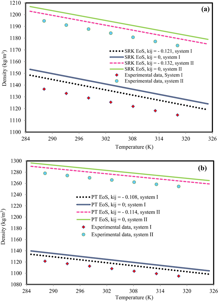
The density behavior of (a) C6mimBr + EGMME (system I: xIL = 0.3990; system II: xIL = 0.7003) and (b) C6mimPF6 + EGMME (system I: xIL = 0.2006; system II: xIL = 0.8019). The experimental data are from Pal and Kumar (Pal and Kumar, 2012).
As another suggestion to model the IL-mixture density, application of semi-empirical equations was studied. The various semi-empirical equations were developed in this communication (see Appendix A). The semi-empirical equation parameters are determined by matching prediction density (based on semi-empirical equation) with experimental data. To model the density of IL-mixture systems based on semi-empirical equations, two methods was considered. In the first method, the coefficients of Eqs. (20) - (24) that were presented by authors (Valderrama and Zarricuetac, 2009; Hosseini et al., 2013) with all mixing rules that are provided in Table 3, was applied. The obtained results indicated presented coefficients was not appropriate idea to predict IL-mixture systems. For instance, Fig. 3 indicates the results of C4mimHSO4 + water at xIL = 0.2066 and C2mimC2SO4 + water xIL = 0.8775 using Eqs. (20) - (24) with available coefficients in the literature (Valderrama and Zarricuetac, 2009; Hosseini et al., 2013). The behavior of all equations is out of experimental data. Indeed, this behavior was predictable. Due to the presented coefficients by authors (Valderrama and Zarricuetac, 2009; Hosseini et al., 2013) were obtained based on pure experimental data.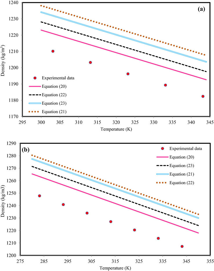
The density behavior of (a) C4mimHSO4 + water, xIL = 0.2066 and (b) C2mimC2SO4 + water, xIL = 0.8775. The experimental data are from Bhattacharjee et al. (Bhattacharjee et al., 2012).
In the second method, the coefficients of Eqs. (20) - (25) was optimized using improved laplacian whale optimization algorithm. ILs composed of various cation structures and due to the behavior of each cation-family is similar, subsequently; to present a comprehensive IL-mixture density model, the semi-empirical equation coefficients of each cation-family were obtained, separately. In order, to obtain the coefficients, 70% of experimental data of each cation-family were used (according to SSMD method) and the rest of them were applied to investigate the accuracy of presented modification. Table 5 indicates the obtained results of coefficients of each cation-family.
BuPy
C2mim
C3mim
C4mim
C6mim
C8mim
Hmim
Mmim
Moim
OcPy
Omim
Eq. (20)
1.4276
1.4333
3.4141
2.5435
1.5269
2.2006
1.2667
1.4437
2.6180
1.6672
1.4351
−24.4288
−12.1559
−16.3907
−20.5247
−18.5703
−25.5447
–22.8585
−19.3457
−17.1898
−27.4722
−25.7281
90.4586
89.7786
96.8990
100.7207
110.7657
91.6898
79.7247
111.2392
101.9145
85.9381
98.3142
−200.1014
−198.2336
−210.2945
−187.1111
−167.4654
−179.7048
−202.6287
−206. 6067
−199.7036
−188.7557
−208.7630
289.1036
375.1405
318.5853
302.9995
297.3273
360.1928
350.1520
325.2051
378.4956
398.9698
341.7952
−265.4304
–222.9168
−238.7594
−274.5659
−205.1692
−297.9199
−301.6974
−269. 9160
−241.8707
−250.9096
−225.3736
79.9026
91.1474
99.8885
86.3146
55.1304
69.2458
92.8226
64.1757
95.4982
79.2156
80.3134
12.2575
10.1718
30.4343
23.3592
20.1003
17.1419
11.2923
9.6965
16.8973
21.0296
15.2065
−125.2630
−140.5759
−145.0790
−150.5398
−134.8022
−120.1509
−138.4204
−145.5454
−124.7027
−117.9474
−115.4756
400.2939
505.1158
477.5352
563.3992
489.2882
471.6863
523.9821
512.4536
469.5230
485.1155
530.7250
−925.9014
−999.6598
−851.6390
−874.8194
−905.6473
−963.5568
−812.2813
−887.7445
−945.4015
−824.9164
−911.4074
1241.7436
1300.4585
1225.7009
1150.4076
1281.2225
1200.4156
1269.2198
1250.3201
1195.2240
1312.8904
1275.3236
−707.6116
−714.8203
−680.4270
−750.7814
−697.3104
−760.1877
−720.8627
−777.6309
−685.1064
−711.8785
−730.7766
177.1086
197.4633
164.1537
185.7426
155.2871
161.8064
149.8930
185.8250
123.4602
201.9203
134.9338
Eq. (21)
1.1278
0.7955
0.8490
1.0164
0.9630
0.9295
1.0516
0.9245
0.9888
1.0989
1.1354
0.9789
0.8439
0.7985
0.8510
1.1044
1.2000
0.7999
1.2331
0.1219
1.1945
1.1182
1.3484
1.6776
1.3846
1.8330
1.8698
1.7689
1.2860
1.3067
1.9288
1.2168
1.7321
−2.3143
−2.6155
−2.4477
−2.5247
−1.9864
−1.9550
−2.7765
−1.8697
−2.5991
−2.1273
−2.2932
1.6046
2.1912
1.7298
1.9164
2.3200
2.3160
1.6645
2.3982
2.5198
2.5117
1.8912
Eq. (22)
0.1704
0.5795
0.9418
0.1931
0.3159
0.5941
0.7740
0.8810
0.7598
0.6996
0.2748
−0.1017
−0.0466
−0.3398
−0.0315
−0.2359
−0.0914
−0.1694
−0.1151
−0.1340
−0.0485
−0.0911
0.1616
0.2553
0.1452
0.1492
0.3222
0.4515
0.2805
0.3075
0.3060
0.3693
0.4205
−0.1258
−0.1900
−0.8515
−0.0369
−0.0239
−0.0760
−0.0427
−0.0710
−0.0232
−0.0564
−0.2085
−0.0431
−0.1971
−0.0895
−0.0472
−0.1643
−0.0712
−0.0977
−0.0832
−0.0353
−0.0595
−0.0504
0.7512
0.9699
1.1848
0.6585
0.8582
1.5507
1.2532
0.9266
0.8858
0.9616
0.9090
1.5863
0.9602
0.8349
1.2209
1.3500
1.3130
1.3322
1.5338
1.6114
1.4690
1.6237
−0.9008
−0.6452
−0.2955
−0.4415
−0.3555
−0.5366
−0.7005
−0.8023
−0.5367
−0.9498
−0.5369
−1.2906
−1.1832
−0.9130
−1.6756
−1.5181
−0.6977
−2.4936
−1.9311
−2.4297
−1.2415
−1.1341
1.1196
1.5928
1.0380
1.4301
1.3295
1.6635
0.8577
1.7030
1.6049
1.6873
1.6685
Eq. (23)
0.9237
0.9546
0.8591
1.0457
1.0078
1.1426
1.0658
1.1769
1.1013
1.0215
0.9991
−1.5944
−1.8065
−1.0305
−1.7807
−1.5123
−1.2685
−1.6932
−1.8750
−1.9345
−1.1633
−1.2911
1.4910
1.1961
1.4801
1.6313
1.7802
1.9290
1.6889
1.5471
1.9232
1.5406
1.5774
−0.5045
−0.9082
−0.5401
−0.8468
−1.2402
−0.7031
−1.2997
−1.3899
−0.6139
−1.4053
−0.9271
0.1691
0.2583
0.8386
0.1172
0.2183
0.1331
0.1459
0.1639
0.2663
0.4048
0.5017
−0.1475
−0.4908
−0.2453
−0.2381
−0.1930
−0.2464
−0.1167
−0.2775
−0.3877
0.2138
0.2800
0.3936
0.6255
0.7937
0.8723
0.9885
0.3403
0.9230
0.5377
0.5324
0.1234
0.3024
−0.0788
−0.0958
−0.4074
−0.0130
−0.0344
−0.0412
−0.0212
−0.0715
−0.0950
−0.0812
−0.1439
−0.0247
−0.0444
−0.5809
−0.0571
−0.0986
−0.0653
−0.0826
−0.0673
−0.0325
−0.0559
−0.0197
0.8583
0.8467
0.9535
0.9651
1.0002
0.9752
0.9736
1.0066
0.9032
1.1348
0.8155
Eq. (24)
0.2460
0.4161
0.4562
0.2525
0.3958
0.3565
0.1419
0.2463
0.3942
0.3905
0.3069
0.1202
0.1873
0.1806
0.1746
0.2739
0.2780
0.1672
0.1348
0.1415
0.3984
0.3195
0.3704
0.3878
0.8206
0.9808
0.4860
0.7096
0.6277
0.7660
0.5270
0.5532
0.2534
0.7872
0.1991
0.4587
0.6378
0.3589
0.3845
0.3397
0.4229
0.8887
0.6658
0.3048
Eq. (25)
0.4359
0.4119
0.4195
0.1330
0.8724
0.0561
0.6827
0.3716
0.6354
0.8796
0.4114
0.7885
0.1887
0.9206
0.6706
0.9045
0.9032
0.1506
0.4059
0.7984
0.6710
0.5605
−0.5214
−0.1829
−0.1358
−0.2606
−0.5895
−0.6440
−0.5259
−0.3548
−0.3120
−0.6672
−0.6436
1.5579
1.7272
1.5768
1.5816
0.8496
2.1506
2.1369
1.5607
20.1661
1.3143
0.8827
The statistical validation of optimized coefficients was investigated by introducing four statistical parameters of correlation factor (R2), average absolute percent deviation (AAPD), standard deviation (STD) and root mean squared error (RMSE). These parameters are formulated as following and the values of them are provided in Table 6.
BuPy
C2mim
C3mim
C4mim
C6mim
C8mim
Hmim
Mmim
Moim
OcPy
Omim
Eq. (20)
R2
0.9843
0.9826
0.9810
0.9672
0.9965
0.9610
0.9850
0.9660
0.9882
0.9817
0.9779
RMSE
0.0151
0.0268
0.0658
0.0235
0.0425
0.0630
0.0409
0.0604
0.0563
0.0634
0.0261
Mse × 103
0.1459
0.4930
0.1256
0.5311
0.3114
0.6735
0.2278
0.1295
0.5176
0.4596
0.3616
AAPD
0.6203
0.1036
0.5026
0.2572
0.3013
0.3208
0.1818
0.0895
0.2943
0.2166
0.2724
STD
1.2825
0.8968
0.7412
0.9432
0.6912
1.2285
0.8310
0.6492
0.5619
0.9588
1.0348
Eq. (21)
R2
0.9694
0.9877
0.9866
0.9665
0.9765
0.9671
0.9622
0.9891
0.9820
0.9889
0.9796
RMSE
0.0490
0.0417
0.0980
0.0186
0.0332
0.0246
0.0678
0.0568
0.0542
0.0178
0.0203
Mse × 103
0.5543
0.2363
0.6750
0.6876
0.3615
0.1061
0.6381
0.1885
0.2560
0.3759
0.2241
AAPD
0.2200
0.3742
0.7296
0.8094
0.2403
0.1911
0.2633
0.2744
0.5545
0.1070
0.4451
STD
0.6077
1.0013
1.3647
0.7242
0.8031
0.7237
1.2732
0.9935
0.9702
0.6824
1.2029
Eq. (22)
R2
0.9648
0.9874
0.9902
0.9611
0.9814
0.9829
0.9879
0.9798
0.9894
0.9969
0.9874
RMSE
0.0602
0.0236
0.0820
0.0465
0.0329
0.0677
0.0191
0.0102
0.0605
0.0515
0.0772
Mse × 103
0.5845
0.1933
0.4885
0.6527
0.2146
0.5924
0.6365
0.1818
0.2674
0.6023
0.2503
AAPD
0.6905
0.1205
0.3155
0.7333
0.2660
0.3034
0.8785
0.2799
0.3015
0.2622
0.1240
STD
0.8942
0.5669
0.4012
0.6171
1.2187
0.6396
1.2972
1.2513
0.5196
0.7305
0.8006
Eq. (23)
R2
0.9780
0.9671
0.9856
0.9683
0.9975
0.9744
0.9727
0.9822
0.9631
0.9927
0.9839
RMSE
0.0243
0.0233
0.0642
0.0660
0.0592
0.0306
0.0114
0.0298
0.0456
0.0598
0.0600
Mse × 103
0.2669
0.1757
0.7953
0.6583
0.5247
0.2842
0.6188
0.4152
0.5709
0.3258
0.1862
AAPD
0.0726
0.6398
0.2103
0.2083
0.2473
0.8620
0.1735
0.0448
0.5440
0.7945
0.9860
STD
0.6415
0.8807
0.6718
1.0162
0.7894
0.9218
0.6626
0.8150
0.7477
0.8000
0.8267
Eq. (24)
R2
0.9834
0.9629
0.9600
0.9725
0.9838
0.9812
0.9793
0.9633
0.9940
0.9865
0.9909
RMSE
0.0168
0.0574
0.0419
0.0217
0.0496
0.0196
0.0622
0.0135
0.0286
0.0589
0.0641
Mse × 103
0.3712
0.2964
0.8294
0.3186
0.2629
0.1378
0.2661
0.3379
0.4493
0.5525
0.6964
AAPD
0.1296
0.1990
0.7658
0.3636
0.4531
0.8402
0.2328
0.2751
0.1893
0.5120
0.0473
STD
0.6227
0.9080
1.0767
1.0769
0.7726
0.8680
0.6457
1.1202
0.5200
0.7332
0.8881
Eq. (25)
R2
0.9874
0.9953
0.9705
0.9864
0.9806
0.9634
0.9818
0.9694
0.9868
0.9850
0.9878
RMSE
0.0529
0.0387
0.0952
0.0571
0.0569
0.0529
0.0282
0.0508
0.0474
0.0142
0.0350
Mse × 103
0.6510
0.2341
0.8651
0.6813
0.3055
0.3780
0.1360
0.4671
0.2850
0.5357
0.2802
AAPD
0.0558
0.6734
0.5588
0.4156
0.9137
0.6346
0.0422
0.2637
0.2711
0.0939
0.6510
STD
1.0151
0.6302
1.0973
0.5869
0.6230
1.1140
0.6719
0.9082
0.8108
1.0359
0.6241
For example, Fig. 4 indicates the total results of the correlation factor based on Eq. (20) and C4mim-family with applying test data subcategories. The solid 45° line shows the details of fitting between the experimental data and the related ones, whereas circles point show the comparison between the obtained results based on Eq. (20) and the experimental density data. The R2 value is 0.9856. Indeed, closeness of the circle points to the solid line in Fig. 4 demonstrates the presented modification technique has acceptable ability to predict IL-mixture density.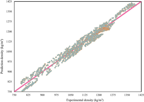
Predicted versus experimental IL density mixtures for test datasets. The reported results are related to Eq. (23) and C4mim-family.
The six semi-empirical equations gave different results and any cation-family presented various results to predict the density of IL-mixture system at all temperatures. For example, Fig. 5 indicates the density behavior of OmimBF4 + ethanol (xIL = 0.247 and xIL = 0.839) and C4mimClO4 + ethanol (xIL = 0.709 and xIL = 0.900) based on semi-empirical equations (using test data). According to Fig. 5, the semi-empirical equations could predict the mixture density with acceptable accuracy. All semi-empirical equations have similar behavior and they could predict the mixture density with acceptable accuracy.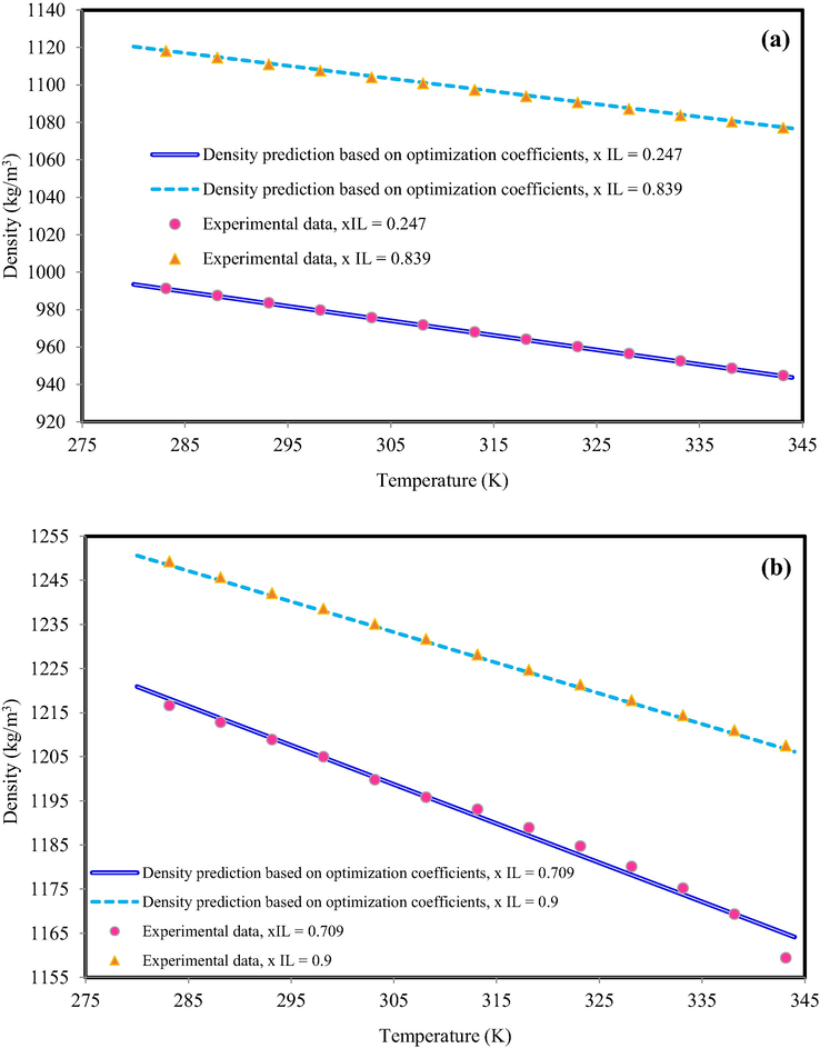
The density behavior of (a) OmimBF4 + ethanol, xIL = 0.247 and xIL = 0.839 (b) C4mimClO4 + ethanol, xIL = 0.709 and xIL = 0.900. The obtained results based on Eq. (20) with optimized coefficients. The experimental data are from Mokhtarani et al. (Mokhtarani et al., 2008).
All semi-empirical equations, except Eq. (24), only were used to predict pure IL density up to now. For first time, we have examined the capability of these equations to predict the density of IL-mixture system at various mole fractions and temperatures. Subsequently, mixing rules had significant role in this development and they show the effect of component mole fraction. According to Table 3 various mixing rules, at least three mixing rules for each property, was investigated. The mixing rule of all thermodynamic properties except acentric factor and critical temperature, was linear. The experimental data density mixture are function of mole fraction and temperature and all semi-empirical equations are function of reduced temperature (Tr), therefore, critical temperature mixing rule have remarkable influence on accuracy of obtained results based on semi-empirical equations. Several critical temperature mixing rules have been investigated but non-linear ones indicated better results. This mixing rule is function of second power of mole fraction and also second order of radical of both IL and solvent critical temperature ( ).
To more investigation of accuracy of obtained confidents, the density behavior of IL binary systems that was unused in the optimization coefficients procedure was model. For instance, Fig. 6 indicates the results of BuPyBF4 + water, xIL = 0.144 and xIL = 0.737 and OcPyBF4 + water, xIL = 0.242 and xIL = 0.816 binary systems. The obtained results indicated the all semi-empirical equation can predict the behavior of density of IL-mixture with satisfactory accuracy and it demonstrates the accuracy of presented models. Furthermore, the values of AAPD of all binary systems are provided in Table 7. According to Table 7, the AAPD of Eqs. (20) - (25), SRK EoS and PT EoS are 0.7312, 0.7666, 0.7631, 0.7583, 0.7750, 0.7560, 22.0470, 18.9372, respectively. Indeed, Eqs. (21) - (23) have almost the similar functionality of temperature and they need the similar input, subsequently, the AAPD of them is almost similar. Also, the results of NM equation are considerable. This equation requires critical temperature, molecular weight and critical volume as input but the temperature functionality of NM equation is contained two different non-linear expressions.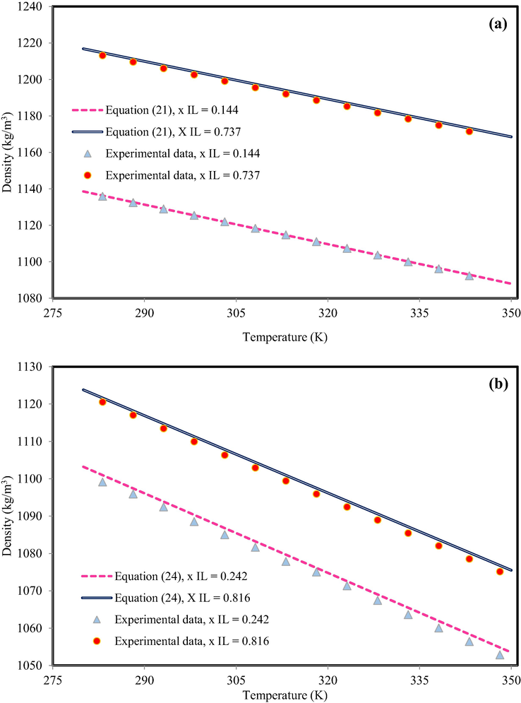
The density behavior of (a) BuPyBF4 + water, xIL = 0.144 and xIL = 0.737 and (b) OcPyBF4 + water, xIL = 0.242 and xIL = 0.816. The experimental data are from Mokhtarani et al. (Mokhtarani et al., 2009).
System number*
Eq. (20)
Eq. (21)
Eq. (22)
Eq. (23)
Eq. (24)
Eq. (25)
SRK EoS
PT EoS
1
0.2366
0.9938
0.6236
0.2660
0.5182
0.1118
20.6262
18.3660
2
0.3138
0.9736
0.4391
0.6749
0.7861
0.9652
22.2795
25.7948
3
0.4822
0.4050
0.5199
0.8488
0.7260
0.3481
17.8561
31.2398
4
0.9775
0.3402
0.3065
0.7040
0.3442
0.8307
19.7477
16.4109
5
0.6457
0.5299
0.1762
0.6311
0.7489
0.3351
24.2136
18.8411
6
0.0599
0.7519
0.4793
0.5294
0.6676
0.2002
17.4252
29.3787
7
0.4855
0.3745
0.2577
0.2571
0.1959
0.3253
19.9113
14.9408
8
0.0024
0.8064
0.5500
0.5801
0.2602
0.7941
22.6095
30.5583
9
0.1135
1.0045
0.4547
0.3476
0.3795
0.8473
28.3839
20.2513
10
0.0138
0.5264
0.8608
0.7882
0.6452
0.3883
17.4518
18.5096
11
0.1767
0.2741
0.4487
0.8825
0.8156
0.6651
24.2974
19.3817
12
0.3506
0.3614
0.5615
0.1624
0.4078
0.4751
20.3464
13.5489
13
0.1209
0.5865
0.1637
0.8849
0.8533
0.8700
30.0776
21.9492
14
0.0255
0.6330
0.4872
0.7121
0.3213
0.7359
18.3771
14.7050
15
1.1136
0.4185
0.9857
0.5823
0.6095
0.8825
22.2321
23.5823
16
1.2179
0.4185
0.7488
0.4786
0.7445
1.1079
15.9280
11.2609
17
0.5172
0.8909
0.8568
0.5696
0.6746
0.7641
14.2380
10.9519
18
0.7567
0.7174
0.7288
0.8311
0.8608
0.4860
17.4102
20.8407
19
1.1845
0.4581
1.3931
0.6394
1.1597
0.6883
25.1026
23.3282
20
0.8233
1.1454
0.7946
0.7233
0.5799
0.7766
16.0869
14.5742
21
0.9013
1.0476
0.3938
1.0127
0.9457
1.0858
17.1235
18.5200
22
0.9249
0.9706
0.4059
0.6363
1.4645
0.8279
20.4922
18.4954
23
1.0355
0.8541
1.0774
0.3261
0.7345
0.9145
21.3880
19.2354
24
0.7399
0.5475
0.8528
1.1006
1.1143
1.1042
13.2281
15.3350
25
0.4353
0.6610
0.6409
0.6654
0.4502
0.4738
25.0577
21.5457
26
0.6793
0.7609
1.1913
0.9286
0.8049
1.3186
18.1603
14.2094
27
0.9769
1.0715
0.9096
1.1884
1.0869
0.5985
19.4429
16.5605
28
0.7649
1.1982
1.1568
0.8768
0.6276
0.5799
23.2291
18.4369
29
0.8012
0.7374
0.8162
0.9983
1.0290
1.0849
17.5259
14.2769
30
1.0510
0.8341
0.4441
1.0620
0.7719
1.1473
15.2965
13.3316
31
0.8245
0.6287
0.9059
0.9214
0.9887
0.6440
20.0022
16.4984
32
0.5583
0.8584
0.8950
1.3014
1.1800
0.9410
23.1882
19.5751
33
0.9300
1.1585
1.0751
0.6562
0.4595
0.7722
16.0683
15.3228
34
0.7717
0.7922
0.8343
0.8596
1.1295
0.9228
22.1401
20.1552
35
0.8754
0.7628
0.6590
1.1077
0.7437
0.6417
21.2102
18.2696
36
0.7837
0.3913
1.1158
0.5664
0.8120
0.4831
25.2277
23.5010
37
0.3936
1.0511
0.6216
0.9803
0.7890
1.2878
22.3686
19.6221
38
0.9286
0.5020
0.7248
0.7647
0.9881
0.5595
20.2726
17.3448
39
0.7720
0.7740
0.5062
1.0887
1.1570
0.8122
24.0508
23.4803
40
0.9569
0.9026
0.7202
0.5310
0.4262
1.2882
25.2024
20.3102
41
1.0547
1.0610
0.9624
0.6344
0.6095
0.7403
19.5668
16.2232
42
0.7944
0.8800
0.7353
0.8147
0.8221
1.1154
15.0228
13.5625
43
1.3939
0.9507
0.5585
1.0797
0.4545
1.3330
20.2113
22.2219
44
0.7020
0.7874
0.9803
0.7192
1.3622
0.8104
17.1145
18.4901
45
0.9286
1.1702
0.6608
1.1069
0.6355
0.6103
23.4376
17.1839
46
0.8677
0.9151
0.8137
0.5581
1.1561
0.7747
16.2416
11.3694
47
1.0205
0.4208
0.7411
0.9023
0.5926
0.5682
18.5587
16.4248
48
0.6093
0.8715
0.8273
0.7207
0.6800
0.6479
22.1217
14.3894
49
1.1242
0.5098
0.5184
1.0568
0.9178
0.9191
20.4540
15.1821
50
0.9328
0.7951
0.7125
0.8855
1.0723
0.7718
26.1576
19.5411
51
1.0071
0.6699
0.9141
1.0862
0.5984
0.6173
17.4104
20.3195
52
1.0873
0.5733
0.7026
0.6897
0.8417
0.7947
20.4437
25.4147
53
0.9315
0.9009
0.4173
0.8277
0.9166
0.8500
26.1834
22.4174
54
0.8387
1.1847
1.1503
0.6041
0.6460
0.6555
27.2895
20.3707
55
0.6351
0.3769
0.8066
0.2743
1.0362
1.3064
19.4910
16.1931
56
1.1824
0.5897
1.2777
0.4010
0.4390
0.7860
30.2903
25.2651
57
0.9700
0.9605
1.4981
0.7703
0.5992
1.0047
20.5929
14.6114
58
0.7653
1.0829
0.7731
1.0306
0.9872
1.2551
24.4616
19.4590
59
0.6842
0.5678
0.8767
0.7822
1.1243
0.5189
22.3143
17.2093
60
0.9165
1.2557
0.7068
0.9975
0.6618
0.8639
28.2994
20.3600
61
1.0381
0.9686
0.5094
0.6778
1.0406
0.8255
25.4474
16.5362
62
0.9058
1.0349
0.7562
0.3886
0.6784
0.7343
17.1212
22.2459
63
0.7250
0.7988
0.9334
0.7909
0.7682
1.1759
20.3667
16.1150
64
0.8682
1.0271
0.7306
1.1561
0.8568
0.6108
31.2142
25.2189
65
0.4962
0.4970
0.5676
0.7679
0.5670
0.8960
19.3296
12.3942
66
1.0135
0.9702
0.6312
1.1071
0.9584
0.5956
22.2232
20.4761
67
0.6528
0.6173
1.0526
0.4040
1.1928
1.3312
32.3213
26.5113
68
1.0590
1.0087
0.9463
1.3112
0.8234
0.9441
23.2044
19.3744
69
0.9628
0.7772
1.2073
0.4152
0.6455
1.1672
25.4590
15.4579
70
0.6561
0.7240
0.8028
0.5473
1.0702
0.7092
26.3738
22.3680
71
0.9642
0.4912
0.7451
1.0189
0.6651
0.5748
20.1293
24.1283
72
0.8688
1.1057
0.9951
0.8658
0.9186
1.0616
19.3760
13.5043
73
1.1162
0.7521
1.1260
1.0728
0.5636
0.9677
26.2362
17.3098
74
0.9265
0.7323
1.0939
0.8414
1.0548
0.3449
29.4522
25.1483
75
0.8010
1.0950
0.9583
0.5727
0.9696
1.0753
26.3080
20.2611
76
0.5967
0.4691
0.8234
1.1601
0.7618
0.5173
22.1527
18.1489
77
0.9746
1.1053
0.9506
0.6131
0.4281
1.1279
18.3662
11.2910
78
1.1670
0.8141
0.6111
1.0475
0.6152
0.9081
20.1981
14.4174
79
0.7856
1.1656
0.7128
0.6545
1.1571
0.9243
27.0376
19.2677
80
0.6580
0.8298
1.0294
0.7007
0.6109
1.1576
16.4658
10.3470
81
1.0063
0.9674
0.9832
0.8751
1.0015
0.9081
25.2930
19.5448
82
0.5515
1.0584
0.7457
0.2872
0.6918
1.0400
23.1865
20.4934
83
1.0324
1.0120
0.6887
0.7416
1.1276
0.8326
22.0761
26.1072
84
0.4616
0.2522
1.1657
0.5994
0.6575
1.1419
19.5836
23.2855
85
1.0995
0.7428
0.8728
1.0030
0.3680
0.6658
17.1113
12.5065
86
0.5938
1.0764
0.9620
1.0255
1.0601
0.8125
20.2285
13.3925
87
1.1246
1.2448
1.1656
0.8523
0.5949
0.4132
23.5275
17.4630
88
0.9295
0.8751
0.5092
1.1403
0.7628
0.3559
16.3271
22.1459
89
0.8602
0.3406
1.0966
0.8856
0.9862
1.0417
26.4708
18.3663
90
1.1492
0.4746
0.8574
1.1516
1.1790
0.4501
17.2814
23.1822
91
0.7055
1.1907
0.5293
0.4263
0.8536
0.9265
26.3938
20.4300
92
1.0513
0.6945
1.0913
0.3350
0.9183
0.4481
20.0959
12.3902
93
0.5322
1.0568
0.8131
0.9647
0.6648
1.0756
18.2427
25.4996
94
0.5131
0.4318
1.2280
0.6211
0.3784
0.7032
20.3507
16.3106
95
0.4457
0.6764
0.9205
1.1251
0.5122
0.3348
27.4560
19.0258
96
1.1939
0.6925
0.5570
0.7361
0.6118
0.6541
30.3385
24.3835
97
0.9260
1.0649
0.8042
0.5577
1.0655
0.5390
20.5021
26.6911
98
0.5716
0.4146
0.7446
0.9852
0.7023
0.4653
23.2957
19.2800
99
1.1555
0.9556
0.9868
1.1887
0.3375
0.8093
24.4195
20.4356
100
0.9246
0.7489
0.8192
0.6692
1.0280
1.1993
19.1761
15.3610
101
0.7495
1.0863
1.2728
1.1763
0.7377
0.7280
25.2438
19.5895
102
0.8335
0.3809
0.9006
0.5686
1.0282
0.5233
20.3450
15.2570
103
1.0173
1.0885
0.7667
0.7837
0.7383
0.3304
26.2945
19.3476
104
0.9434
1.1998
1.0156
1.0830
0.8712
0.9216
23.3907
20.4538
105
1.0471
0.1241
0.0436
0.1824
0.3021
1.1070
19.6531
14.7969
106
0.4073
0.6530
0.0282
0.7868
0.9569
0.8697
22.9742
17.6829
107
0.2090
0.6049
0.9676
0.3350
0.5228
0.2784
26.1503
20.5382
108
0.7435
0.9946
0.5816
0.2269
0.8929
0.3780
23.6544
18.8334
109
0.2463
0.7650
0.6785
0.6209
0.4821
0.7939
17.3563
13.3656
110
0.4968
0.6024
0.2164
0.1852
0.6014
0.5938
24.5270
20.9553
111
0.8723
0.9480
0.8896
1.0091
0.7773
0.9340
16.4367
11.7906
112
0.7836
0.5759
0.4184
0.6427
0.7976
0.4819
27.6427
23.4184
113
0.2562
0.8570
0.1923
0.7249
0.3573
0.1481
21.3660
17.5832
114
0.3278
0.1728
0.4784
0.2393
1.0286
0.8061
20.1862
22.8198
115
0.2654
0.5318
1.0878
0.6776
0.8433
0.2049
30.2989
24.8862
116
0.1344
0.1149
0.7160
0.3176
0.1619
0.4388
28.2236
23.3719
117
0.4082
1.1505
0.5350
1.1786
1.4210
0.6877
23.4463
17.2598
118
1.0533
0.4865
0.6443
0.7387
0.3543
0.8803
21.2917
15.3503
119
0.7894
0.9125
0.9461
0.9538
0.7117
1.0629
18.5784
23.5890
120
0.1277
0.8769
0.3354
0.7117
0.9756
0.7431
26.8781
20.6559
121
0.3077
0.7126
0.4122
0.4314
0.8272
0.9128
24.3818
19.3874
122
0.4527
0.4187
0.6633
1.0881
1.1240
0.3716
25.7595
18.2520
123
0.7520
0.2798
0.8228
0.3768
1.0647
0.3627
18.2413
13.3981
124
0.6198
0.9099
1.1055
0.9867
0.6933
0.5579
23.3374
19.1641
125
0.4934
0.3213
0.8309
0.4075
0.6011
0.5841
30.3836
24.2541
126
0.8331
0.8488
0.5991
0.9630
1.1515
0.3296
19.1895
14.7146
127
0.1512
1.1110
1.0555
1.1976
0.4223
0.9994
27.5462
23.5352
128
1.0881
0.6283
0.3094
0.5494
0.9735
0.1587
18.6711
15.2730
129
0.0558
0.9169
0.8610
0.7337
0.4125
0.5869
20.4749
16.4600
130
0.3635
0.7954
0.6822
0.8151
0.9161
1.0103
23.1087
20.3927
Average AAPD
0.7312
0.7666
0.7631
0.7583
0.7750
0.7560
22.0470
18.9372
In the case of density mixtures, as mentioned, influence of mixing rule to extend the critical properties and molecular weight is significant and it affect the accuracy of semi-empirical equation. According to Table 3, different mixing rules were applied to generalize the pure thermodynamics properties to binary mixtures. After investigation the accuracy and comparison the AAPD values of obtained results, the final mixing rules for each thermodynamics properties were selected. For example, the obtained results of C2mimBF4 + acetone binary system at xIL = 0.5772 and xIL = 0.8304 based on equation (25) and C2mimBF4 + dimethylsulphoxide binary system at xIL = 0.3417 and xIL = 0.6717 based on equation (23) are presented in Fig. 7. The optimization process was performed based on both final and linear mixing rules (
). According to Fig. 7, the selection of mixing rules had considerable effect on the optimized coefficient and furthermore, prediction of density of IL-mixture.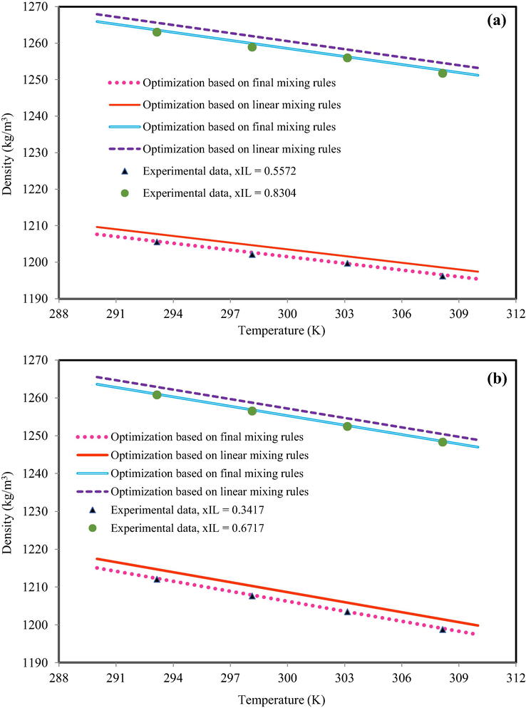
The density behavior of (a) C2mimBF4 + acetone, xIL = 0.5772 and xIL = 0.8304 based on equation (25) and (b) C2mimBF4 + dimethylsulphoxide, xIL = 0.3417 and xIL = 0.6717 based on equation (23). The experimental data are from Bhagour et al. (Bhagour et al., 2013).
4 Conclusion
In the present communication, six semi-empirical equations with various mixing rules was employed to calculate the density of 130 different IL-mixture binary systems. The considered systems covered 51 ILs (11 cation-family) and 41 solvents. The used semi-empirical equations had unknown coefficients and to present comprehensive IL-mixture density, the unknown coefficients was obtained using laplacian whale optimization algorithm for each cation-family, separately. Regarding the presentation in the field of cost function, the obtained results were highly accurate. To obtained of unknown coefficients, 70% of experimental data of each cation-family according to SSMD method were used and the remaining experimental data were applied to investigate the accuracy of presented models. The obtained results based on both test and train data were acceptable and the performed modification on semi-empirical equations to generalize binary mixture was successful. Beside the semi-empirical equations, capability of SRK EoS and PT EoS cubic equations state to was investigated predict IL-mixture density; however, the obtained results based on both CEoSs had significant deviation from experimental data therefore, that using binary interaction parameter could not decrease deviation, remarkably.
Declaration of Competing Interest
The authors declare that they have no known competing financial interests or personal relationships that could have appeared to influence the work reported in this paper.
References
- Arab. J. Chem.. 2021;14:103164
- Arab. J. Chem.. 2020;13:9090.
- Arab. J. Chem.. 2021;14:102909
- J. Phys. Chem. C.. 2016;120:8704.
- J. Mol. Liq.. 2021;336:116581
- Ind. Eng. Chem. Res.. 2014;53:9506.
- Ind. Eng. Chem. Res.. 2009;48:11189.
- Arab. J. Chem.. 2020;13:5821.
- J. Chem. Eng. Data.. 2019;64:3316.
- Korean J. Chem. Eng.. 2017;34:2686.
- Green Energy Environ.. 2020;5:303.
- Chem. Chem. Technol.. 2019;13:1.
- J. Chem. Eng. Data.. 2019;64:594.
- J. Mol. Liq.. 2017;236:172.
- ACS Energy Lett.. 2016;1:21.
- Appl. Therm. Eng.. 2020;181:115943
- Chem. Eng. Sci.. 2020;227:115927
- Particuology.. 2021;57:201.
- Phys. Chem. Chem. Phys.. 2003;5:4869.
- Fluid Phase Equilibr.. 2009;275:145.
- J. Chem. Eng. Data.. 2010;55:4114.
- J. Solution Chem.. 2011;40:1528.
- J. Solution Chem.. 2013;42:979.
- J. Chem. Thermodyn.. 2013;57:203.
- Thermochim. Acta.. 2013;556:75.
- J. Phys. Chem. B.. 2013;117:12535.
- J. Mol. Liq.. 2014;200:160.
- Phys. Chem. Chem. Phys.. 2015;17:26918.
- J. Solution Chem.. 2013;42:1854.
- J. Mol. Liq.. 2009;149:66.
- Ind. Eng. Chem. Res.. 2010;49:4420.
- Ind. Eng. Chem. Res.. 2011;50:7027.
- Chem. Eng. Sci.. 2011;66:2690.
- Ind. Eng. Chem. Res.. 2012;51:10274.
- J. Phys. Chem. B.. 2012;116:9089.
- Ind. Eng. Chem. Res.. 2012;51:758.
- Ionics. 2012;18:769.
- Fluid Phase Equilibr.. 2015;395:51.
- J. Mol. Liq.. 2020;308:113027
- Comput. Chem. Eng.. 2010;34:2085.
- Chem. Eng. Sci.. 2019;3:100026
- Int. J. Refrig.. 2016;69:418.
- Ind. Eng. Chem. Res.. 2019;58:12787.
- J. Chem. Thermodyn.. 2008;40:84.
- Fluid Phase Equilibr.. 2021;531:112908
- J. Supercrit. Fluid. 2008;47:109.
- Fluid Phase Equilibr.. 2017;447:39.
- AICHE J.. 2021;63:17194.
- Ind. Eng. Chem. Res.. 2002;41:5510.
- Chemistry Open.. 2021;10:216.
- J. Chem. Thermodyn.. 2010;42:852.
- Chem. Eng. Sci.. 2017;159:58.
- Ind. Eng. Chem. Res.. 2019;58:4277.
- J. CO2 Util.. 2017;21:162.
- J. Phys. Chem. Ref. Data.. 2006;35:1475.
- Fluid Phase Equilibr.. 2021;531:112898
- J. Chem. Phys.. 2020;153:104101
- Ind. Eng. Chem. Res.. 2008;47:1318.
- PVT and phase behaviour of petroleum reservoir fluids. Elsevier; 1998.
- Perry's chemical engineers' handbook. McGraw-Hill Education; 2019.
- J. Chem. Thermodyn.. 2009;41:323.
- J. Chem. Thermodyn.. 2012;45:43.
- Fluid Phase Equilibr.. 2009;285:83.
- J. Chem. Thermodyn.. 2013;56:123.
- J. Chem. Thermodyn.. 2013;60:76.
- J. Chem. Eng. Data.. 2012;57:3473.
- Fluid Phase Equilibr.. 2011;305:114.
- J. Solution Chem.. 2007;36:631.
- J. Chem. Thermodyn.. 2012;51:51.
- J. Chem. Eng. Data.. 2006;51:2145.
- J. Chem. Thermodyn.. 2011;43:800.
- Chin. Chem. Lett.. 2012;23:1295.
- J. Chem. Eng. Data.. 2007;52:1468.
- Int. J. Thermophys.. 2009;30:1491.
- J. Chem. Eng. Data.. 2009;54:1110.
- J. Chem. Thermodyn.. 2008;40:949.
- J. Chem. Thermodyn.. 2009;41:888.
- J. Chem. Thermodyn.. 2016;99:40.
- J. Solution Chem.. 2006;35:311.
- J. Chem. Thermodyn.. 2012;44:121.
- J. Chem. Eng. Data.. 2008;53:677.
- J. Mol. Liq.. 2013;177:301.
- J. Chem. Thermodyn.. 2010;42:640.
- J. Chem. Thermodyn.. 2013;64:1.
- J. Chem. Thermodyn.. 2013;57:238.
- Colloids Surf. A Physicochem. Eng. Asp.. 2012;404:1.
- J. Chem. Eng. Data.. 2008;53:596.
- J. Chem. Thermodyn.. 2007;39:291.
- J. Chem. Eng. Data.. 2009;54:2307.
- J. Mol. Liq.. 2011;163:128.
- J. Mol. Liq.. 2010;154:41.
- Thermochim. Acta.. 2012;527:211.
- J. Mol. Liq.. 2012;169:156.
- J. Chem. Thermodyn.. 2012;48:129.
- Fluid Phase Equilibr.. 2012;334:157.
- J. Chem. Thermodyn.. 2011;43:796.
- J. Chem. Eng. Data.. 2006;51:696.
- J. Chem. Thermodyn.. 2014;74:103.
- J. Chem. Thermodyn.. 2014;71:236.
- J. Mol. Liq.. 2013;177:54.
- J. Therm. Anal. Calorim.. 2016;123:785.
- J. Chem. Thermodyn.. 2012;47:300.
- J. Chem. Thermodyn.. 2006;38:651.
- J. Chem. Thermodyn.. 2007;39:978.
- J. Chem. Thermodyn.. 2012;47:203.
- J. Mol. Liq.. 2018;261:174.
- Chem. Eng. Sci.. 1984;39:357.
- Chem. Rev.. 1949;44:233.
- Chem. Eng. Sci.. 1972;27:1197.
- Fluid Phase Equilibr.. 1993;91:87.
- Ind. Eng. Chem. Fundam.. 1976;15:59.
- High Energ. Dens. Phys.. 2018;28:7.
- J. Mol. Liq.. 2019;281:490.
- Chem. Eng. Sci.. 2018;192:565.
- J. Supercrit. Fluid. 2010;55:846.
- Comput. Part. Mech.. 2019;6:721.
- Chem. Eng. Sci.. 2021;229:116045
- Chem. Eng. Sci.. 1980;35:1503.
- Chem. Eng. Sci.. 1982;37:463.
- Fluid Phase Equilib.. 2020;508:112433
- Arab. J. Chem.. 2021;14:103123
- Ind. Eng. Chem. Res.. 1991;30:2576.
- Fluid Phase Equilibr.. 2004;224:157.
- AIChE J.. 1971;17:1341.
- AIChE J.. 1979;25:653.
- B. E. Poling, J. M. Prausnitz, J. P. O’connell, The properties of liquids and gases. New York. 2001.
- Chemical, biochemical, and engineering thermodynamics. John Wiley & Sons; 2017.
- Thermodynamic models for industrial applications: from classical and advanced mixing rules to association theories. John Wiley & Sons; 2009.
- Fluid Phase Equilibr.. 1998;153:231.
- Chem. Eng. Data.. 2014;59:571.
- Fluid Phase Equilibr.. 1983;13:91.
- Sci. Total Environ.. 2020;716:137007
- Atmos. Res.. 2018;213:450.
- Eur. J. Agron.. 2018;98:65.
- Neurocomputing.. 2019;328:5.
- Arab. J. Geosci.. 2018;11:1.
- Measurement.. 2021;167:108288
- Machine learning for dummies. John Wiley & Sons; 2021.
- Curr. Opin. Chem. Biol.. 2008;12:366.
- Technometrics. 1969;11:137.
- Water Resour. Manag.. 2019;33:905.
- Chemometr. Intell. Lab.. 1996;33:35.
- Eng. Manag. J.. 2019;10:713.
- Adv. Eng. Softw.. 2016;95:51.
- Sensors.. 2018;18:2674.
- Artif. Intell. Rev.. 2006;26:159.
- Knowl. Eng. Rev.. 1997;12:341.
- Int. J. Remote Sens.. 2018;39:2784.
Appendix A
The list of all semi-empirical equations that are used in this study, are given in Table A.1.
Model
Parameters
,
,
,
,
,
,
,
,
,
,
,
,
,
,
,
,
,
,
,
,
,
,
,
,
,
,
,
,
,


