Lumped kinetic model for degradation of chitosan by hydrodynamic cavitation

2.1 Materials

Chitosan (deacetylation degree > 90%) was obtained from Kabo Industrial Co., Ltd. (Shanghai, China). Acetic acid (CH₃COOH) and sodium acetate (CH₃COONa) were purchased from Chengdu Kelong Chemical Reagent Factory. Glucan was purchased from Waters, USA. Deionized water was provided with a conductivity of 4 μs/cm.

2.2 Instruments

The experimental analysis was measured with a Waters gel permeation chromatograph equipped with an Ultrahydrogel column (Milford, Massachusetts, USA), 2414 refractive index detector and 1515 pump. The hydrodynamic cavitation field was generated in a home-made reactor equipped with a magnetic pump (1/2DW-750, rated voltage/power: 200 V/750 W, Zhejiang Aolong Technology Development Co., Ltd. China) and pressure guages (0.6 Mpa, Hangzhou Guanshan Instrument Co., Ltd. China).

2.3 Methods

Fig. 1 shows the schematic of the experimental setup for hydrodynamic cavitation. It consists of a closed-loop system. The chitosan solution was drawn from a tank, and transferred into the impinging reactor and jet cavitation reactor with two magnetic pumps through the values V₁, V₂ and V₃. Then, the solution was discharged into the tank. In the reactors, jet cavitation was generated by using a Venturi tube, which is illustrated in Fig. 2.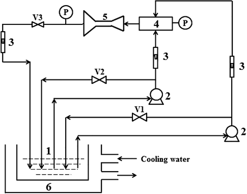

Close

Fig. 1

Schematic presentation of the experimental setup for hydrodynamic cavitation. 1-holding tank; 2-magnetic pump; 3-rotameter; 4-impinging reactor; 5-jet cavitation reactor; 6-cooling water; V1, V2, V3-valve.

Export to PPT

Close

Fig. 2

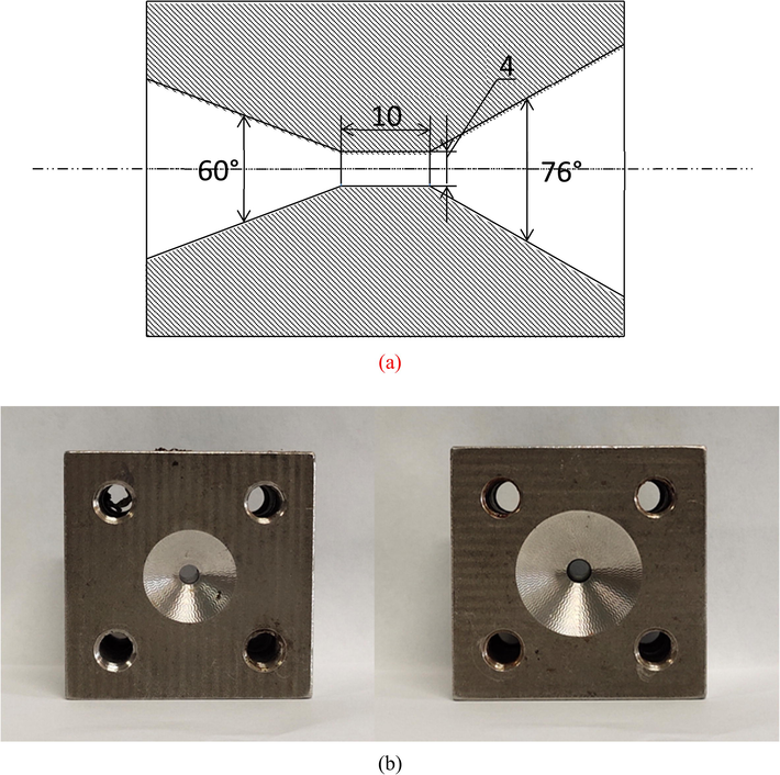
Structure of Venturi tube (a) Photograph of Venturi setup (b).

Export to PPT

The optimized chitosan degradation conditions adopted in this experiment were found by Huang et al. (2015). 3 L of a 3 g/L chitosan solution (pH = 4.4; contained 0.2 mol/L CH₃COOH and 0.1 mol/L CH₃COONa) was poured into the tank. The magnetic pumps were initiated. The reactions were performed for 120 min, and samples were withdrawn every 5 min, under the conditions of pH of 4.4, and inlet pressure of 0.4 Mpa (adjusted by the valves V₁ and V₂). The experiments were performed at different temperatures (30 °C, 35 °C, 40 °C, 45 °C, 50 °C and 60 °C). The inlet and outlet angles of the Venturi tube in the hydrodynamic cavitation device were adjusted to be 60 °and 76°, and the length and diameter of the throat were measured to be 10 and 4 mm.

2.4 Characterization

The molecular weights and its distributions of the products were measured by gel permeation chromatography (GPC) with a mobile phase comprising 0.2 mol/L CH₃COOH and 0.1 mol/L CH₃COONa and a flow rate of 0.6 mL/min (Moore, 1964). 25 μL sample was detected with the sensitivity of 32 under detector and column temperatures of 30 °C. The glucan standard was used to calibrate the molecular weights of chitosan samples (Ren et al., 2006).

After the degradation by hydrodynamic cavitation, the concentrations of degradation products were quantified by GPC with a five-point calibration curve (0.9, 1.2, 1.5, 1.8, and 2.1 mg/mL) (Lee and Chang, 1996).

3.1 Models establishment

Before the establishment of models, some hypotheses necessary are presented as follows:

1. The degradation of chitosan follows the first-order reaction kinetics.

2. Chitosan degradation products with similar molecular weights have similar kinetic characteristics in the reaction system. The lumps were divided according to the molecular weights of products. The components in a lump do not interact with each other.

3. The lump with high molecular weights can be degraded into another lump with low molecular weights. The lowest lump will not be degraded anymore. The reaction rates of different lumps are different. Moreover, no reverse reactions take place.

4. The reactions take place in a homogeneous solution, so the influence of molecular diffusion will be ignored.

5. The hydrodynamic cavitation degradation of chitosan agrees with the rules of random degradation.

The lumps were divided by their molecular weights which are one of the most important parameters of chitosan, because the kinetic properties will be affected by the molecular weights. For example, oligochitosan has certain inhibitory effects on fungi and microorganisms when the average molecular weights were in the range of 5 kDa ∼ 10 kDa (Kyoon No et al., 2002). The oligochitosan with molecular weights of 1.5 kDa and 3 kDa showed excellent water solubility (Mourya et al., 2011), moisture absorption, moisture retention and other properties (Xia et al., 2011). The whole system should be subdivided according to the physiological activities before the appropriate lump number was determined.

The reaction system was divided into n lumps based on the hypotheses. The network established is shown in Fig. 3. In this reaction network, molecular weights decrease from A₁ to A_n. If the reaction of each step exists, the number of reactions (N_r) equals n(n-1)/2. Building on the hypotheses and the n-lumped reaction network, the differential equations representing the reactions of these lumps are shown as follow:

Close

Fig. 3

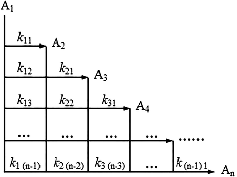
Reaction network for n lumps.

Export to PPT

As mentioned before, there are n(n-1)/2 reactions. Since each reaction contains a reaction rate constant k_ij, a total of n(n-1)/2 parameters are unknown. The equations are mass balances.

3.2 Trade-off of the number of lumps

The whole degradation system was divided into 12 lumps according to the analysis results in section 3.1. The molecular weights of A₁ to A₁₂ are above 1000 kDa, 800 kDa ∼ 1000 kDa, 500 kDa ∼ 800 kDa, 300 kDa ∼ 500 kDa, 200 kDa ∼ 300 kDa, 100 kDa ∼ 200 kDa, 80 kDa ∼ 100 kDa, 50 kDa ∼ 80 kDa, 30 kDa ∼ 50 kDa, 10 kDa ∼ 30 kDa, 5 kDa ∼ 10 kDa, and below 5 kDa. The concentrations of degradation products at different times are shown in Table 1. The changing trends of mass concentrations over time are shown in Fig. 4(a). The concentrations of lumps A₃, A₄ and A₅ increased first, and then decreased slowly, showing similar kinetic behaviors. Same phenomenons were observed in the profiles of lumps A₉ and A₁₀, A₁₁ and A₁₂. The lumped kinetics research method combines components into certain groups, of which the kinetic behaviors are similar. The number of variables and parameters can be reduced and a complicated system can be simplified (Shi et al., 2005). Based on these fundamental principles of lumped kinetics and experimental results, eight-lumped model was obtained by combing the above lumps with similar kinetic behaviors.

Close

Fig. 4

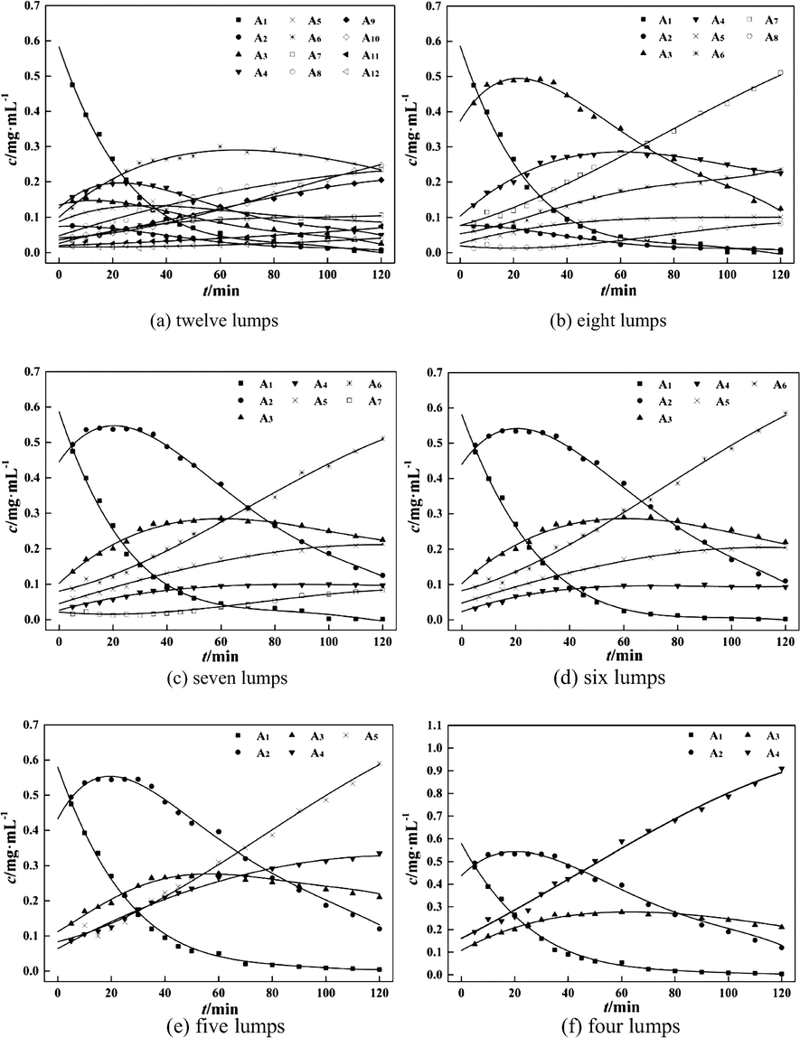
Chitosan degradation curves for different lumps line-calculated value; dot-experimented value; t-degradation time; c-product concentration.

Export to PPT

According to the above-mentioned strategy, the eight-lumped model can be further merged into seven-lumped, six-lumped, five-lumped and four-lumped models. The fitting results and corresponding RSS values of these models are shown in Fig. 4(b)∼(f) and Table 2. Among these models, the eight-lumped and six-lumped models, with the RSS values of 5.18 × 10⁻³ and 5.36 × 10⁻³, exhibited better performances. The number of unknown kinetic parameters k_ij in the six-lumped model (15) was much smaller than those in the seven-lumped and eight-lumped models. For the four-lumped and five-lumped models, the RSS values were large, and the molecular weight ranges of products in all the lumps were too large, which may decrease the accuracy of parameters estimated. In the sections below, the six-lumped kinetic model was taken into account.

3.3 Six-lumped kinetic model and parameters estimation

3.3.2

3.3.2 Estimation of lumped kinetic parameters

The degradation reactions were performed at 30, 40, 50 and 60 °C, and the products concentrations at different times were determined, as shown in Table 3.

Table 3 Chromatographic quantitative analysis results for degradation products at 30 °C at different time.

t/min	Concentration/mg·mL−1						cA/mg·mL−1
	A1 lump	A2 lump	A3 lump	A4 lump	A5 lump	A6 lump
0	0.5909	0.4316	0.1111	0.0278	0.0457	0.0908	1.2979
5	0.4773	0.4960	0.1396	0.0347	0.0560	0.0904	1.2939
10	0.3969	0.5361	0.1677	0.0430	0.0701	0.1345	1.3483
15	0.3357	0.5437	0.1825	0.0473	0.0772	0.1105	1.2970
20	0.2690	0.5434	0.1991	0.0524	0.0858	0.1248	1.2745
25	0.2186	0.5434	0.2189	0.0589	0.0970	0.1456	1.2824
30	0.1627	0.5401	0.2498	0.0702	0.1186	0.1747	1.3160
35	0.1286	0.5231	0.2642	0.0765	0.1310	0.2079	1.3314
40	0.0972	0.4840	0.2666	0.0789	0.1369	0.2252	1.2889
45	0.0740	0.4498	0.2700	0.0823	0.1446	0.2419	1.2626
50	0.0627	0.4317	0.2786	0.0870	0.1554	0.2623	1.2777
60	0.0403	0.3863	0.2930	0.0970	0.1794	0.3202	1.3161
70	0.0224	0.3201	0.2817	0.0980	0.1865	0.3540	1.2628
80	0.0151	0.2793	0.2792	0.1018	0.1993	0.3944	1.2692
90	0.0085	0.2277	0.2663	0.1025	0.2081	0.4576	1.2707
100	0.0039	0.1830	0.2543	0.1045	0.2203	0.4961	1.2619
110	0.0026	0.1474	0.2344	0.1018	0.2233	0.5503	1.2598
120	0.0009	0.1211	0.2243	0.1026	0.2328	0.5958	1.2775

Note: c_A is the sum of the concentration of six lumps.

The estimation values of reaction rate parameters and the comparison of experimental and calculation values at different temperatures are shown in Table 4 and Fig. 5. It can be seen that the reaction rate constants in the degradation of different lumps into other lumps were rather different.

Table 4 Parameters estimation results and fitting error of lumping model.

k/min−1	Temperature°C				Relative error/%	Temperature/oC
	30	40	50	60		30	40	50	60
k11	3.69 × 10−2	4.09 × 10−2	5.98 × 10−2	1.63 × 10−1	A1 lump	−12.85	−18.14	–22.42	−30.56
k12	6.54 × 10−3	1.07 × 10−3	1.39 × 10−6	2.17 × 10−12	A2 lump	−4.67	−1.27	−12.31	−14.50
k13	3.49 × 10−3	5.86 × 10−8	6.14 × 10−5	5.61 × 10−12	A3 lump	−4.76	−0.07	−1.29	−10.90
k14	2.68 × 10−3	4.56 × 10−11	3.99 × 10−6	2.01 × 10−11	A4 lump	−13.08	−1.18	2.09	−6.23
k15	2.66 × 10−3	9.11 × 10−9	8.05 × 10−6	2.22 × 10−14	A5 lump	−7.39	−0.71	0.78	−14.82
k21	9.64 × 10−3	1.30 × 10−2	2.37 × 10−2	7.73 × 10−2	A6 lump	−4.64	−1.43	−0.29	−0.46
k22	1.08 × 10−3	2.85 × 10−3	2.67 × 10−3	4.37 × 10−7
k23	3.56 × 10−3	3.97 × 10−3	3.13 × 10−3	1.12 × 10−3
k24	3.07 × 10−3	9.45 × 10−8	1.86 × 10−3	1.11 × 10−2
k31	4.83 × 10−4	1.27 × 10−3	1.28 × 10−2	6.19 × 10−2
k32	1.78 × 10−3	2.11 × 10−3	9.65 × 10−3	3.78 × 10−2
k33	9.47 × 10−3	1.26 × 10−2	8.87 × 10−3	1.93 × 10−3
k41	7.08 × 10−8	1.69 × 10−3	3.94 × 10−2	1.59 × 10−1
k42	1.01 × 10−9	6.55 × 10−3	1.35 × 10−8	2.34 × 10−14
k51	1.70 × 10−3	3.38 × 10−3	2.72 × 10−2	1.02 × 10−1

Close

Fig. 5

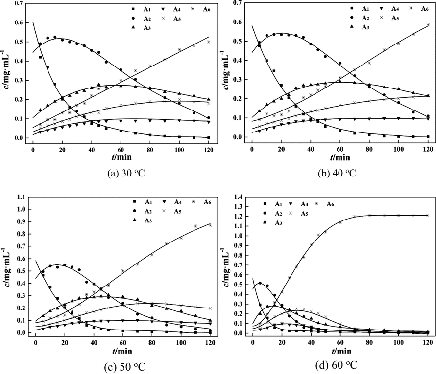
Chitosan degradation curves at different temperatures. line-calculated value; dot-experimented value; t-degradation time; c-product concentration.

Export to PPT

For example, the reaction rate constants in the degradation of A₁ and A₂ into A₃, A₄, A₅ and A₆ were different. Under the condition of same degradation time, the reaction rate constants k₁₃, k₁₄, and k₁₅ are relatively small in the degradation of A₁ with a greater molecular weight, while those (k₂₂, k₂₃, and k₂₄) are relatively large in the degradation of A₂ with a smaller molecular weight. In addition, the reaction rate constants k₁₁, k₂₁, k₃₁, k₄₁ and k₅₁ are large in the whole degradation process. The results illustrated that the degradation of chitosan mainly occurred on the diagonal of the six-lumped reaction network, and the reactions followed the path: A₁ → A₂ → A₃ → A₄ → A₅ → A₆. This result may be caused by the chemical and mechanical effects in the hydrodynamic cavitation process. These effects led to different fracture sites in chitosan chains. The chemical effect led to random cuts and mechanical effect led to central cuts. As for the central cut, the cleavage took place at the middle points of the chitosan chains, and degradation products with larger molecular weights were prone to form. In random cuts, each linkage of the chitosan molecular chain had the same cleavage probability. It can be seen that the lump A₁ was more likely to degrade into lump A₂ rather than lumps A₃, A₄, A₅, and A₆ (Yan et al., 2020a). At 60 °C, the values k₁₂, k₁₃, k₁₄, k₁₅ were low. This is probably because after the temperature reached a certain value, the coefficient of viscosity and surface tension of the solution decreased, and the vapor pressure of the solution increased. The cavitation threshold decreased, and cavitation bubbles were easily produced. However, with the increase of temperature, the vapor pressure increased faster compared to the temperature of solution. The transient high temperature and high pressure generated by the collapse of cavitation bubbles decreased, reducing the intensity of cavitation, weakening the degradation rate. The similar situation was also observed by Huang et al. (2015) in the process of chitosan degradation. These results showed that the degradation reactions of chitosan led to the formation of lumps with similar molecular weights.

Analysis results in Table 4 indicate that six-lumped model was well fitted to the experimental values at different temperatures. The errors of fitting results at 30 °C, 40 °C and 50 °C were small, especially those at 40 °C. The results showed that the six-lumped kinetic model can well-describe the distribution of degradation products of chitosan by hydrodynamic cavitation.

It can be seen from Fig. 5(a)–(d) that the concentrations of lump A₁ with the largest molecular weight declined over time at different degradation temperatures. The degradation rates of lump A₁ increased with the increase of temperatures. In contrast, the concentrations of lump A₆ with the lowest molecular weight increased over time at different degradation temperatures, and the formation rate of lump A₆ was accelerated significantly with the increase of temperatures. At the early stages of the reactions, the formation rates of lumps A₂ and A₃ were higher than the degradation rates of A₂ and A₃, leading to the increase of their concentrations. With the proceeding of the degradation reactions, the concentrations of lumps A₂ and A₃ declined because the degradation rates surpassed the formation rates. The concentrations of lumps A₄ and A₅ showed an increasing trend at 30 and 40 °C, while they first increased and then decreased at 50 and 60 °C. The main reason could be that at low temperatures such as 30 and 40 °C, the degradation rates of all the lumps were relatively low. With the increase of temperature, the degradation reactions were accelerated. The degradation reactions reached a high level in a short time, and the degradation degree of chitosan was higher.

Fig. 5(d) shows that at 60 °C, the lumps A₁, A₂, A₃, A₄ and A₅ almost completely degraded after 70 min of reactions, and the mass concentration of lump A₆ tended to be constant. The results show that the reaction rates could be obviously improved by increasing the temperatures of reactions. A higher temperature facilitated the degradation process (Huang et al., 2013). The degradation temperature and degradation time were vital to the degradation of chitosan. Products with medium molecular weights were obtained at lower reaction temperatures or shorter reaction time, while products with low molecular weights were obtained at higher reaction temperatures or over longer reaction time. In summary, the composition and distribution of chitosan degradation products can be controlled by adjusting the reaction time and temperature.

3.4 Activation energy results of lumped reactions

The correlations between reaction rate constants lnk and 1/T corresponding to the points on the diagonal of the six-lumped reaction network at 30 ∼ 60 °C are illustrated in Fig. 6. The correlations were in good accordance with the Arrhenius equation, and the corresponding activation energy values were calculated to be 40 ∼ 399 kJ·mol⁻¹. The corresponding equations are given as follow:

Close

Fig. 6

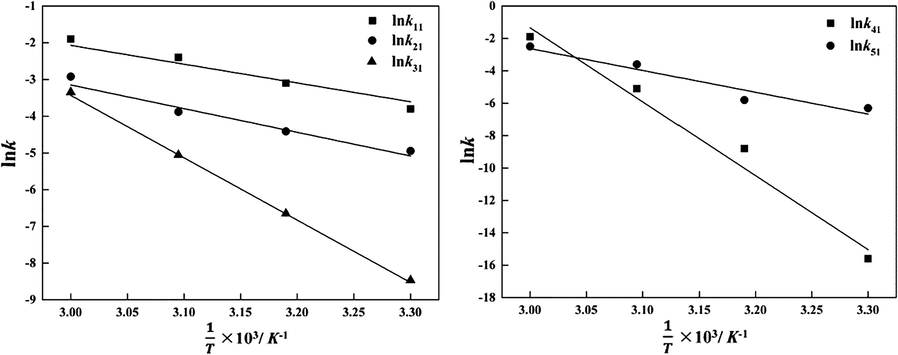
Reaction rate constants with temperature. T-temperature; k-reaction rate constants.

Export to PPT

3.5 Prediction ability of the model

The prediction ability of the model and reliability of kinetic parameters obtained by fitting were assessed by comparing the fitting results with data derived in other experiments under different degradation reaction conditions. The degradation reactions were carried out at 35 and 45 °C, and the samples were withdrawn at 0, 8, 16, 24, 32, 42, 55, 65, 75, 85, 95, 105, 115, 120 min.

The values calculated and measured are depicted in Tables 5 and 6. Most of the average absolute deviations were < 9.3%, except the prediction deviation for the lump A₁. The large deviation for the lump A₁ may be due to that the degradation products contained chitosan with molecular weights beyond the detection range of the gel permeation chromatograph. Another reason may be that the range of molecular weights of chitosan in the lump A₁ was large, resulting in different kinetic properties of certain products. In addition, the large number of parameters could also increase the errors for the rate constant estimated. The average absolute deviations for lumps A₂, A₃ and A₆ were < 3%, and those for A₄ and A₅ were slightly larger. The reason is that the degradation rates of chitosan were low at 35 °C and 45 °C, and the lumps A₄ and A₅ did not completely degrade. The analysis results indicated that multi-parameter lumped kinetic models can quantitatively predict the degradation process of chitosan and concentration distribution of lumped components in the reaction networks.

References

- Numerical Methods with Chemical Engineering Applications in MATLAB. England: Cambridge University Press; 2006.
- Modeling of cavitation as an advanced wastewater treatment. Desalin. Water Treat.. 2013;51:1609-1614.
- [CrossRef] [Google Scholar]
- A review of cleaner intensification technologies in biodiesel production. J. Clean. Prod.. 2017;146:181-193.
- Cleaner production of methyl ester using waste cooking oil derived from palm olein using a hydrodynamic cavitation reactor. J. Clean. Prod.. 2016;112(5):4505-4514.
- Intensification of biodiesel synthesis from waste cooking oil (palm olein) in a hydrodynamic cavitation reactor: effect of operating parameters on methyl ester conversion. Chem. Eng. Process.. 2015;95:235-240.
- Effective photocatalytic removal of selected pharmaceuticals and personal care products by elsmoreite/tungsten oxide@ZnS photocatalyst. J. Environ. Manage.. 2020;270:110870
- Practical computer simulation of chemical processes : MATLAB’s applicat (first ed.). China: Chemical Idustry; 2004.
- Synergistic degradation of chitosan by impinging stream and jet cavitation. Ultrason. Sonochem.. 2015;27:592-601.
- Degradation of chitosan by hydrodynamic cavitation. Polym. Degrad. Stab.. 2013;98:37-43.
- Degradation of Ibuprofen in Aqueous Solution with UV Light: the Effect of Reactor Volume and pH. Water. Air. Soil Pollut.. 2016;227:194.
- Parameter estimation of a six-lump kinetic model of an industrial fluid catalytic cracking unit. Fuel. 2019;235:1436-1454.
- Enzymatic production and biological activities of chitosan oligosaccharides (COS): A review. Carbohydr. Polym.. 2005;62:357-368.
- A review of chitin and chitosan applications, Reactive & Functional Polymers. Reactive Functical Polym.. 2000;46:1-27.
- Antibacterial activity of chitosans and chitosan oligomers with different molecular weights. Int. J. Food Microbiol.. 2002;74(1–2):65-72.
- Polymer molecular weight characterization by temperature gradient high performance liquid chromatography. Polymer. 1996;37(25):5747-5749.
- Optimum conditions for the precipitation of chitosan oligomers with DP 5–7 in concentrated hydrochloric acid at low temperature. Process Biochem.. 1999;34:493-500.
- Photodegradation of Oxytetracycline in the Presence of Dissolved Organic Matter and Chloride Ions: Importance of Reactive Chlorine Species. Water. Air. Soil Pollut.. 2019;230:235.
- Antifungal activity of chitooligosaccharides against the dermatophyte Trichophyton rubrum. Int. J. Biol. Macromol.. 2015;77:330-335.
- Gel permeation chromatography. I. A new method for molecular weight distribution of high polymers. J. Polym. Sci. Part A Gen. Pap.. 1964;2:835-843.
- Chitooligosaccharides: Synthesis, characterization and applications. Polym. Sci. - Ser. A. 2011;53:583-612.
- Gamma radiation degradation of chitosan for application in growth promotion and induction of stress tolerance in potato (Solanum tuberosum L.) Carbohydr. Polym.. 2019;210:289-301.
- Advancement on modification of chitosan biopolymer and its potential applications. Int. J. Biol. Macromol.. 2020;152:681-702.
- Study on homogeneity of enzymatic degradation of chitosan as biomaterials by gel permeation chromatography. Chinese J. Chromatogr.. 2006;24:407.
- Chitin and chitosan: Properties and applications. Prog. Polym. Sci.. 2006;31(7):603-632.
- Lumping kinetic study on the process of tryptic hydrolysis of bovine serum albumin. Process Biochem.. 2005;40:1943-1949.
- Effect of molecular weight of chitosan and its oligosaccharides on antitumor activities of chitosan-selenium nanoparticles. Carbohydr. Polym.. 2020;231
- Study of the depolymerization behavior of chitosan by hydrogen peroxide. Carbohydr. Polym.. 2004;57:31-37.
- Degradation of chitosan by swirling cavitation. Innov. Food Sci. Emerg. Technol.. 2014;23:188-193.
- Biological activities of chitosan and chitooligosaccharides. Food Hydrocoll.. 2011;25:170-179.
- Study on mechanism of chitosan degradation with hydrodynamic cavitation. Ultrason. Sonochem.. 2020;64:105046
- Degradation of chitosan with self-resonating cavitation. Arab. J. Chem.. 2020;13(6):5776-5787.
- Chitosan solution enhances both humoral and cell-mediated immune responses to subcutaneous vaccination. Vaccine. 2007;25:2085-2094.
- Upgrading of crude oil in supercritical water: A five-lumped kinetic model. J. Anal. Appl. Pyrol.. 2017;123:56-64.
- Lumping kinetic model of enzymatic hydrolysis of protein of silkworm pupae-alcalase system. Ciesc J.. 2011;62(09):2588-2594.
- Advances in characterisation and biological activities of chitosan and chitosan oligosaccharides. Food Chem. 2016;190:1174-1181.