

Translate this page into:
QSAR modeling, molecular docking and molecular dynamic simulation of phosphorus-substituted quinoline derivatives as topoisomerase I inhibitors
⁎Corresponding author. mouad.lahyaoui@usmba.ac.ma (Mouad Lahyaoui)
-
Received: ,
Accepted: ,
This article was originally published by Elsevier and was migrated to Scientific Scholar after the change of Publisher.
Abstract
As they facilitate the cleavage of single and double stranded DNA to relax supercoils, unwind catenanes, and condense chromosomes in eukaryotic cells, Topoisomerase plays crucial roles in cellular reproduction and DNA organization. Because the unrepaired single and double stranded DNA breaks these complexes generate might result in apoptosis and cell death, they are cytotoxic agents.
In this study, 28 compounds derived from phosphorus-substituted quinoline are subjected to a quantitative structure–activity relationship (QSAR) using partial least squares, principal component regression, and multiple linear regression. The Gaussian 09 software and the Molecular Operating Environment program were used to calculate molecular descriptors. The anti-proliferative activity was correlated with a variety of electronic and structural characteristics of the molecules, such as EHOMO (energy of the highest occupied molecular orbital) and ELUMO (energy of the lowest unoccupied molecular orbital), which provided evidence for the modeling. The B3LYP/6-31G (d, p) level of theory's Density Functional Theory (DFT) approach was used to compute these electronic properties, and Principal Component Analysis (PCA) was used to test for collinearity between the descriptors. In fact, three alternative prediction models were created using various 2D and 3D descriptor counts, and they were each assessed using the statistical metrics of coefficient of determination (R2) and root mean squared error (RMSE). A MLR model had the best predictive performance of all the constructed models, as indicated by R2 and RMSE of 0.865 and 0.316, respectively.
Three proteins (6G77, 2NS2, and 5K47) for lung, ovarian, and kidney malignancies showed strong binding affinities via hydrophobic interactions and H-bonds with the pertinent chemicals by crystal structure modeling. Compounds C11, C19 and C26, respectively, showed the highest binding energy for ovarian, kidney and lung cancer. The outcomes of the molecular dynamic MD simulation diagram were produced to support the molecular docking findings from earlier research, which demonstrated that inhibitors were stable in the active sites of the selected proteins for 10 ns. This raises the possibility that these chemicals could serve as a valuable model for the development and synthesis of more effective anticancer prospects.
Keywords
QSAR
Quinoline derivatives
PLS
MLR
DFT method
Molecular docking

1 Introduction
Cancer is a complicated condition that develops when cells proliferate uncontrollably under the influence of environmental and genetic factors, invading nearby organs and tissues and metastasizing to form new tumors (Suzuki et al., 2013). It is predicted that by 2030, there may be 21.7 million new cases of cancer and 13 million deaths from it because of the rising global population and average life expectancy (Torre et al., 2012). By preventing DNA synthesis, drugs having cytotoxic effects are effective at delaying cell disclosure, causing the growth rate of cancer cells to be less than their mortality rate. Any intervention that attempts to slow this growth is extensive because cancer cells proliferate considerably more quickly than healthy cities do (Fekri et al., 2019; Exposito et al., 2019; Istifli et al., 2019). Viewed from afar, lung cancer continues to be the most frequently diagnosed cancer for several decades (American Cancer Society, 2018; Bray et al., 2018). According to estimates, 2.1 million new cases of lung cancer were diagnosed in 2018, making up 12% of all cancer cases worldwide (American Cancer Society, 2018; Bray et al., 2018). As a result, efforts to create cytotoxic medications are increasing.
Numerous substances, both naturally occurring and synthesized, include quinoline rings, which are known to be adaptable heterocyclic compounds with a variety of reported pharmacological actions (Abou-Dobara et al., 2019; El-Sonbati et al., 2019). Examples include antimalarial (Aguiar et al., 2018), anti-rheumatoid arthritis (Schrezenmeier and Dörner, 2020), anti-SRAS-Cov-2 (Colson et al., 2020), antimicrobials (Katariya et al., 2020; Orhan Puskullu et al., 2020), antiparasitic (J. Sopková-de Oliveira Santos, P. Verhaeghe, J.-F. Lohier, P. Rathelot, P. Vanelle, S. J.A.C.S.C.C.S.C. Rault, Quinoline derivatives: potential antiparasitic and antiviral agents, 63(11), 2007), anti-tuberculosis (Borsoi et al., 2020), antidiabetic (Taha et al., 2019), anti-inflammatory (Gao et al., 2020), antioxidant (Orhan Puskullu and Tekiner, 2013), anticancer (Mohamed and Ramadan, 2020), anti-arthritic (Sloboda et al., 1991), and analgesics (Boteva et al., 2019). Molecular docking and quantitative structure–activity relationship (QSAR) are two computational tools that have made it feasible to produce pharmaceuticals more quickly, affordably, and effectively (Surabhi and Singh, 2018).
A QSAR study was conducted to correlate descriptors with lung cancer activity expressed as IC50 values, which is the concentration of test compounds needed to reduce the cell survival fraction to 50% of control. These were converted to IC50 negative logarithms (pIC50) to establish a linear relationship with the independent variables. The foundation of QSAR computing techniques involves applying statistical data analysis techniques to quantitatively associate molecular descriptors with a macroscopic object (physical–chemical property or biological activity) for a variety of related chemical substances (Lahyaoui et al., 2023). Its objective is to allow the structural data to be analyzed in order to identify the key determinants of the property or activity being measured. A key issue in the QSAR model building process today is how to achieve a model that is able to clearly predict the activity or property of a novel chemical (Yousefinejad and Hemmateenejad, Dec. 2015).
While employing the QSAR model to create new compounds with improved prediction of pharmacological efficacy that could be useful future drug targets, molecular docking assesses the binding affinity of docked molecules with receptors via the scoring functions of mathematical algorithms. Both methods can be employed independently or together and are well known to be particularly effective in silico drug development. However, the lung, ovarian, and kidney protein malignancies, respectively, were put through a molecular docking investigation to observe the binding mode of phosphorus-substituted quinoline derivatives bearing anticancer action in vitro on the active site of 6G77, 2NS2, and 3IG7.
2 Materiel and methods
2.1 Experimental data
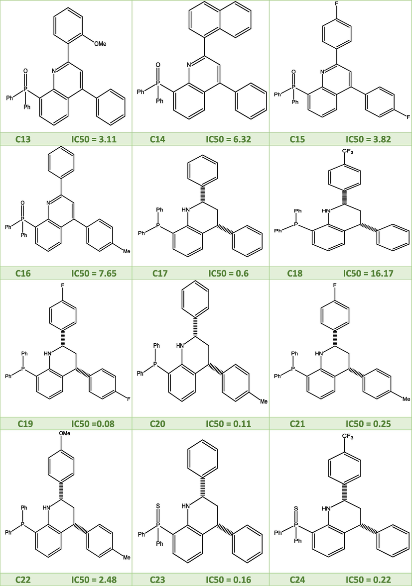
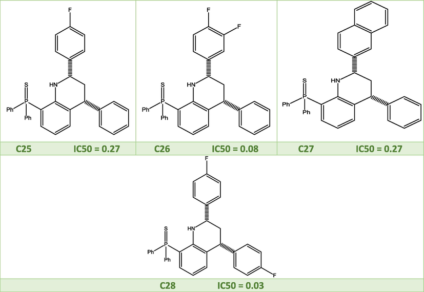
Fig. 1 depicts a series of quinoline compounds that were created by Concepcion Alonso et al (Alonso et al., 2018), who also tested the effectiveness of topoisomerase I inhibitors against human tumor cell line in vitro (lung A549).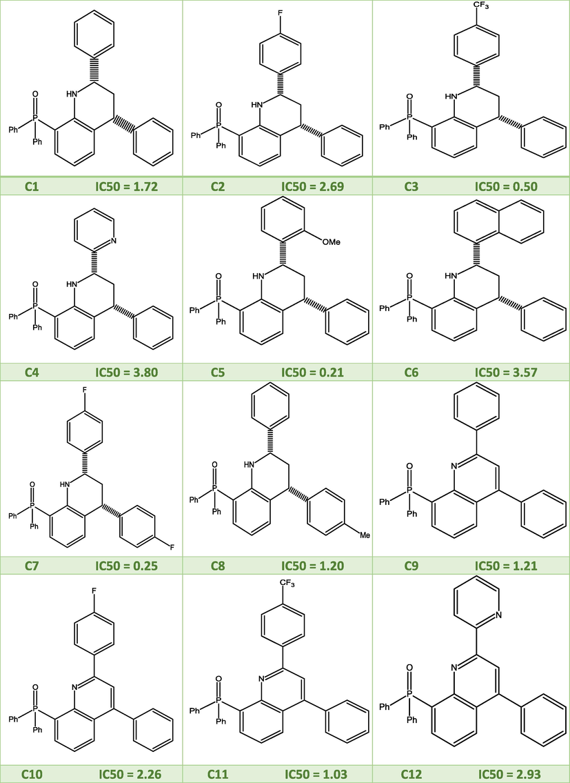
2D molecular structures of the studied quinoline derivatives.
2D molecular structures of the studied quinoline derivatives.
2D molecular structures of the studied quinoline derivatives.
2.2 Molecular descriptors
Obtaining a statistically robust model relies heavily on the ability of the descriptors, derived from a logical and mathematical procedure (Danishuddin, Aug. 2016), to express the variation of activity with structure. The nature of the information quantified by the descriptors generally depends on the type of molecular representation and the algorithm developed for calculating and predicting the correlation between the 28 derivatives and their antiproliferative activity.
The 28 structures were submitted to the Gaussian 09W software using the DFT method based on B3LYP/6–31 G (p, d) to find a geometry where the energy is minimal (Becke, 1992; Becke, 1988; Lee et al., 1988; Adnani and Benjelloun, 2014; El Assiri and Driouch, 2018, 2019; Reda and Saffaj, 2020). This was evaluated based on the minimum energy of the molecular structures, which is established by the absence of imaginary frequencies and by relating the relevant bond lengths and dihedral angle values to reference values. Fig. s1 shows the final optimized geometries.
The same software is also used for the extraction of a set of four quantum-chemical descriptors, namely the energies of the most occupied molecular orbital HOMO and the least vacant orbital LUMO, the total energy of the molecule (Et) and the dipole moment. However, the nature of the currently used descriptors and the degree of encryption of the structural molecular properties linked to some specific physical properties are the core of any QSAR study (Danishuddin, Aug. 2016). Moreover, in order to correlate the inhibition activity with the chemical structures of the studied compounds, the MOE program was also used to calculate the other molecular descriptors and the results have been reported in the annex 3. The QSAR relationship is built by statistical methods such as PLS, PCR and MLR to provide a representation of the QSAR models.
2.3 Statistical analysis
In an effort to build a QSAR model, we picked a set of 28 compounds from previous work that have been reported to have a strong anti-proliferative activity. The XLSTAT program randomly split the entire set into two subsets: a training set (22 compounds) to create the model and a test set (6 compounds) to assess the validity of the created model. the proposed approach involves the use of a principal component analysis (PCA) technique, which checks for redundancy and collinearity between the descriptors studied (Software, 1987; Hmamouchi et al., 2014; Wold et al., 1987; David and Jacobs, 2014) and carries out a comparative statistical study between three mathematical models namely partial least squares regression (PLS), principal component regression (PCR) and multiple linear regression (MLR); with the view of relating activity to molecular structure. After performing the calculations, and using XLSTAT software, version 2014. The selected descriptors were used to establish statistical models that relate the activity of the compounds to their chemical structures by separating the dataset into a training set, which are used to establish the three models and a test set that are exploited to evaluate the performance of these obtained models.
2.4 External validation
The fundamental phase in QSAR analysis is model calculation, but it is not sufficient to ensure the model's validity; it is crucial to assess the model's capacity to forecast new compounds (external validation). Additionally, it is crucial to confirm that the model was not created by chance. In the present test, we implement the QSAR models developed to predict the activities of the compounds in the test set. The latter contains compounds from the series of molecules studied in this work, but not contributed to the development of the QSAR models. The external ability of the QSAR models to predict the activity of the test set molecules was evaluated by calculating the R2 coefficient between the observed pIC50 values and the predicted pIC50 values after addition of the test set. Globarikh and Tropsha (Golbraikh and Tropsha, 2002) reported the usefulness of assessing the value of the R2 test in the external validation of QSAR models. Under this description, when the R2 test value is greater than 0.5, the model is statistically acceptable for prediction and can be implemented for new external data (Chtita, 2021).
2.5 Molecular docking methodology
Molecular Operating Environment (MOE) software was used to calculate and report the scores that were achieved during the molecular docking procedure. Utilizing ChemDraw, the molecular structures were developed (18.2). The target crystal structures for lung (RSK4 N-terminal Kinase Domain in Complex with AMP-PNP, PDB code = 6G77), ovarian (Human spindlin1, PDB code = 2NS2), and kidney cancer (Human Polycystin-2/PKD2 TRP channel, PDB code = 5 K47) were retrieved and created using the Protein Data Bank (https://www.rcsb.org/pdb/welcome.do). All the water-binding cofactors and ligands were separated from the protein structure in order to achieve optimization, and they were subsequently fixed with hydrogen atoms. Selectively removing the active sites to create false atoms. It was switched to assign all parameters and charges to the MMFF94x force field. The MOE site search module was used to set up the alpha site spheres, and the MOE dock module was used to dock the structural model of the molecules to the surface of the cancer protein inside. The dock scoring in the MOE program was carried out using the London dG scoring function, and the upgrading was then performed using two unrelated refining techniques. The top ten dock poses that were chosen for analysis to acquire the high score were then allowed to have self-turning docks. The docking postures were then matched with the ligand in the co-crystallized structure using the database browser, and the RMSD of the docking pose was obtained. Then, to categorize the binding affinity of the compounds to the investigated protein molecules, the binding free energy and hydrogen bonds between the produced molecules and the amino acid residues of the receptors were computed. The default-docking model was defined as the interaction types as with the RMSD of the (native) ligand in the receptor structure.
2.6 Molecular dynamic
During molecular dynamics (MD) simulations to determine the molecular recognition between the ligand and the protein, the three best-docked ligands with the highest activity were selected based on the results of molecular docking (Gholami Rostami and Fatemi, 2018; Er-rajy and El fadili, M., Imtara, H., Saeed, A., Ur Rehman, A., Zarougui, S., Abdullah, S.A., Alahdab, A., Parvez, M.K., Elhallaoui, M. , 2023; Mousavi and Fatemi, 2019; Gholami Rostami and Fatemi, 2019). The GROMACS 5.0 program was used to run MDs for 10 ns. The MD simulation in explicit solvation was performed using the SOC water model (Stouten et al., 2006). Additional input parameters were chosen, including the type of triclinic box, the salt to be neutralized (Na+, Cl), and the SOC water model (Ghosh et al., 2021). Using canonical NVT and isobaric NPT settings, the system was equilibrated at 300 K and 1 bar of pressure, respectively (Schmidt et al., 2009). The MD simulations were run for 10 ns with steady temperature and pressure, a 2 fs time step, and a 1 nm threshold for long-range interactions (El fadili, M., Er-Rajy, M., Kara, M., Assouguem, A., Belhassan, A., Alotaibi, A., Mrabti, N.N., Fidan, H., Ullah, R., Ercisli, S. , 2022).
3 Results and discussion
3.1 Principal component analysis (PCA)
PCA is a qualitative statistical analysis approach used to make a large data set smaller and uncorrelated. These new variables are known as principal components. It allows the practitioner to reduce the number of variables and make the information less redundant. Therefore, in this work, a PCA was performed on the fourteen descriptors with the molecular concentration of the twenty-eight molecules. The nine principal components obtained are presented in Fig. 2.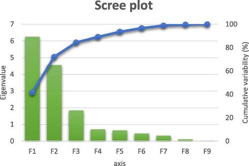
The principal components and their variances.
The contributory of each descriptor to the principal components F1, F2, and F3 were summarized in Table 1. From these results, the descriptors EHOMO, EL-H, I and ƞ show the largest contributions to F1, while the descriptors, ELUMO, A and dipole possess the largest contributions to F2, whereas the descriptors logP(o/w) and lip_acc present the most significant contributions to F3.
F1
F2
F3
correlation
contribution
correlation
contribution
correlation
contribution
E LUMO
0.143
1.65%
0.977
13.74%
−0.073
1.66%
E HOMO
−0.955
11.03%
0.169
2.38%
−0.229
5.21%
E l-h (ev)
−0.883
10.20%
−0.435
6.12%
−0.148
3.37%
KierFlex
−0.718
8.30%
0.124
1.75%
0.372
8.47%
logP(o/w)
−0.393
4.54%
−0.133
1.87%
0.765
17.39%
μ
−0.683
7.89%
0.686
9.65%
−0.224
5.10%
S
−0.788
9.11%
−0.377
5.31%
−0.164
3.74%
χ
0.683
7.89%
−0.686
9.65%
0.224
5.10%
I
0.955
11.03%
−0.169
2.38%
0.229
5.21%
A
−0.143
1.65%
−0.977
13.74%
0.073
1.66%
η
0.883
10.20%
0.435
6.12%
0.148
3.37%
dens
−0.247
2.85%
−0.540
7.60%
0.406
9.22%
dipole
−0.171
1.98%
−0.760
10.70%
−0.324
7.37%
lip_acc
0.462
5.34%
−0.451
6.35%
−0.658
14.95%
Based on the projecting of the variables in the plane of the first three principal components F1, F2 and F3 and their percentage contribution in the two correlation circles shown in Fig. 3, these axes represent 84.44% of variance that is sufficient to describe the information represented by the data set.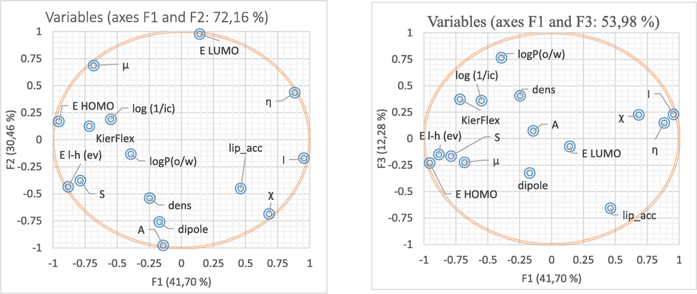
Correlation circles between the principle compounds F1–F2 and F1–F3.
Following the completion of the PCA, the desired descriptors Elumo, Ehomo, KierFlex, logP (o/w), dens, dipole, lip_acc, and S have been selected as inputs for the development of QSAR models by several techniques, including MLR. The eight descriptors mentioned above are retained among fourteen based on the values of the correlation coefficients. In addition, the descriptors having the lowest correlation coefficients between them are selected as shown in the correlation matrix presented in Table 2. Finally, the resulting database is divided into two sets (training and test). This division is performed randomly using the XLSTAT program.
Variables
pIC50
E LUMO
E HOMO
E l-h
KierFlex
logP (o/w)
μ
S
χ
I
A
η
dens
dipole
lip_acc
pIC50
1
E LUMO
0.045
1
E HOMO
0.441
0.048
1
E l-h
0.342
−0.550
0.808
1
KierFlex
0.541
0.011
0.598
0.493
1
logP (o/w)
0.267
−0.238
0.203
0.310
0.478
1
μ
0.377
0.602
0.826
0.335
0.484
0.028
1
S
0.250
−0.477
0.712
0.877
0.421
0.195
0.300
1
Χ
−0.377
−0.602
−0.826
−0.335
−0.484
−0.028
−1.000
−0.300
1
I
−0.441
−0.048
−1.000
−0.808
−0.598
−0.203
−0.826
−0.712
0.826
1
A
−0.045
−1.000
−0.048
0.550
−0.011
0.238
−0.602
0.477
0.602
0.048
1
Η
−0.342
0.550
−0.808
−1.000
−0.493
−0.310
−0.335
−0.877
0.335
0.808
−0.550
1
Dens
0.077
−0.518
0.057
0.353
0.299
0.330
−0.246
0.384
0.246
−0.057
0.518
−0.353
1
Dipole
−0.103
−0.724
0.121
0.528
−0.065
−0.002
−0.311
0.264
0.311
−0.121
0.724
−0.528
0.232
1
lip_acc
−0.536
−0.303
−0.381
−0.140
−0.485
−0.653
−0.475
−0.072
0.475
0.381
0.303
0.140
−0.050
0.447
1
3.2 Partial least square PLS
Quantitative assessment of the compounds by improving the structure–activity relationship was also viewed using partial least squares. The correlation coefficient (R2), MSE and RMSE were used to evaluate and validate the developed model.
pIC50 = − 0.42–0.24 * ELUMO + 0.08 * EHOMO + 0.50 * KierFlex − 0.43 * logP (o/w) + 3.40 * dens + 0.01 * dipole − 0.94 * lip_acc − 0.51 * S
N = 22; R2 = 0.789; MSE = 0.093; RMSE = 0.305
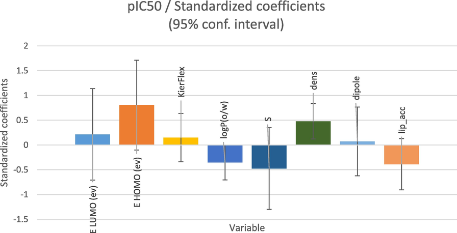
The role that the selected descriptors play in the developed model is very imperative and these have been graphically represented in Fig. 4.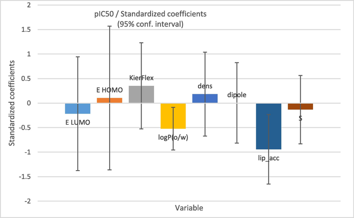
Standardized coefficients versus variables in the proposed PLS model.
The statistical values observed for PLS indicated that the developed model proved to be reliable and predictive as shown in Table 3. In addition, the undifferentiated distribution of residuals on both sides of zero as shown in Fig. 5 revealed that the developed model had no relative inaccuracy. The calculated R2 for PLS indicated that the predicted pIC50 matched well with the observed pIC50, which demonstrates the reliability of the developed model (Fig. 6) Table 4.
Source
DF
Sum of squares
Mean squares
F
Pr > F
Model
7
7.58
1.083
7.472
0.001
Error
14
2.029
0.145
Corrected Total
21
9.608
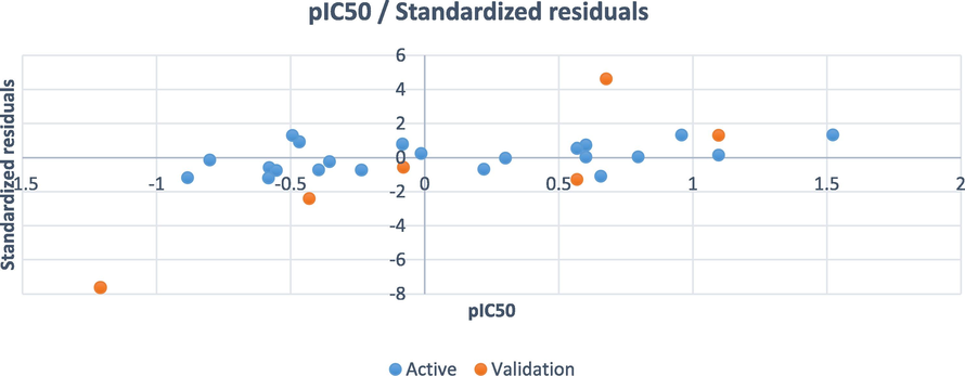
The residuals against observed pIC50.
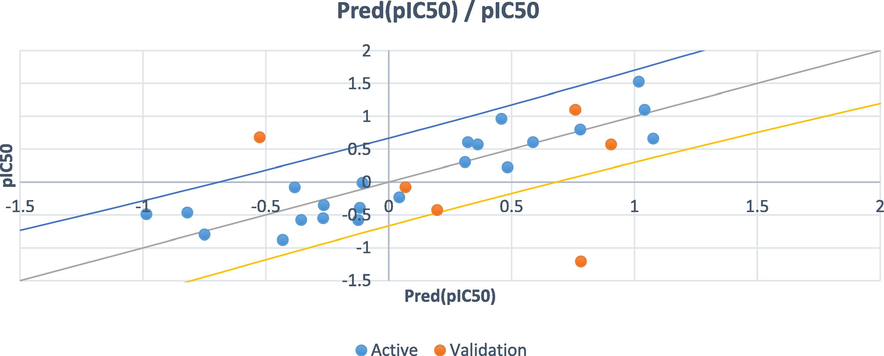
Experimental vs. calculated pIC50 obtained by the PLS model.
compounds
pIC50
PLS model
PCR model
MLR model
Pred (pIC50)
Residual
Pred (pIC50)
Residual
Pred (pIC50)
Residual
1
−0.236
0.043
−0.279
−0.187
−0.048
−0.251
0.016
2
−0.430
0.197
−0.627
0.162
−0.591
0.038
−0.468
3
0.301
0.311
−0.010
0.296
0.005
0.306
−0.005
4
−0.580
−0.355
−0.225
−0.327
−0.253
1.585
−2.165
5
0.678
−0.510
1.187
0.247
0.431
−0.341
1.019
6
−0.553
−0.266
−0.287
−0.235
−0.317
−0.491
−0.062
7
0.602
0.322
0.280
0.367
0.235
0.290
0.312
8
−0.079
0.066
−0.145
−0.046
−0.033
−0.196
0.117
9
−0.083
−0.382
0.299
−0.362
0.763
−0.531
0.448
10
−0.354
−0.263
−0.091
−0.578
0.224
−0.293
−0.062
11
−0.013
−0.106
0.094
0.111
−0.124
−0.086
0.073
12
−0.467
−0.819
0.352
−0.839
0.372
−0.544
0.077
13
−0.493
−0.985
0.493
−0.369
−0.124
−0.459
−0.033
14
−0.801
−0.748
−0.052
−0.800
0.000
−0.617
−0.184
15
−0.582
−0.124
−0.458
−0.139
−0.393
−0.064
−0.518
16
−0.884
−0.431
−0.453
−0.680
−0.203
−0.611
−0.273
17
0.222
0.484
−0.262
0.330
−0.109
0.453
−0.231
18
−1.209
0.796
−2.004
0.831
−2.451
1.081
−2.289
19
1.097
0.762
0.335
0.855
0.242
1.106
−0.009
20
0.959
0.459
0.500
0.467
0.465
0.514
0.445
21
0.602
0.588
0.014
0.718
−0.116
0.771
−0.169
22
−0.394
−0.117
−0.277
−0.155
−1.350
0.438
−0.832
23
0.796
0.780
0.016
0.774
0.513
0.774
0.022
24
0.658
1.077
−0.419
1.311
−0.654
1.132
−0.474
25
0.569
0.901
−0.332
0.620
−0.051
1.010
−0.441
26
1.097
1.042
0.055
0.902
0.195
1.206
−0.109
27
0.569
0.362
0.206
0.239
0.330
0.371
0.198
28
1.523
1.018
0.505
0.932
0.591
1.186
0.337
3.3 Principal components regression (PCR)
In order to boost the quality of the prediction between activity and molecular structure, the selected descriptors were used to evaluate a principal component regression PCR. Their equation obtained along with the statistical parameters calculated using the following ANOVA table is expressed in as:
pIC50 = − 2.46 + 0.50 * ELUMO + 0.37 * EHOMO + 0.22 * KierFlex − 0.19 * logP(o/w) + 6.22 * dens − 0.56 * dipole − 0.13 * lip_acc + 1.29 * S
N = 22; R2 = 0.789; R2adj = 0.683; MSE = 0.145; RMSE = 0.381
The analysis of variance results are summarized in ANOVA Table 3:
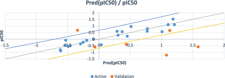
The statistical results obtained by PCR show good quality and improved prediction of activity as well as PLS. It is qualified by quite significant values of the coefficient of determination (R2 = 0.789) and adjusted coefficient of determination (R2adj = 0.683) and low value of MSE 0.147. The resulting values of the predicted pIC50 are adjusted with the experimental pIC50 in Fig. 7.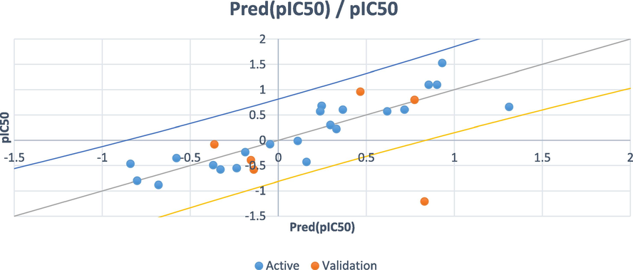
Experimental vs. Calculated pIC50 obtained by the PCR model.
In order to improve the relationship between the predicted activities obtained by the QSAR models developed via PLS, PCR techniques and the eight molecular descriptors; a new QSAR model developed using the MLR technique.
3.4 Multiple linear regression (MLR)
Based on the MLR method, four criteria are used: the coefficient of determination (R2), the coefficient of fit (R2adj), the root mean square error (RMSE) and the Fisher ratio value (F). The outcomes of the MLR that contain the corresponding standardized coefficients of the descriptors and the correlation between the observed and predicted activities are provided in Figs. 8 and 9 respectively. In addition, the established model is represented by the following equation with the statistical parameter values.
pIC50 = − 2.95 + 0.25 * ELUMO + 0.68 * EHOMO + 0.25 * KierFlex − 0.36 * logP(o/w) − 1.83 * S + 9.98 * dens + 0.13 * dipole − 0.41 * lip_acc
N = 22; R2 = 0.865; R2adj = 0.783; RMSE = 0.316; F = 10.448
- Modeling characterization by the normalized coefficients.
- The correlation between the observed and the predicted activities.
Following the coefficient normalization plot, we saw that the built model had three most important descriptors (EHomo, S and dens) correlated with pIC50. The high value of the coefficient of determination (R2 = 0.865), the lower value of the mean square error (MSE = 0.100) and the high value of the statistical confidence (F = 10.448), indicate that the QSAR model is statistically acceptable. Also, the obtained p-value, which is less than 0.05 (Pr less than 0.0002) points out that the QSAR model equation is statistically significant with a level higher than 95%. In Fig. 9, we remark that the distribution of observed and predicted pIC50 values are significantly correlated, which is a result of the low MSE value obtained. In this way, it is clear that the experimentally obtained values and the values predicted by the QSAR model are correlated.
To check the reliability of the predictive ability of the obtained QSAR models, we proceed to an external validation. In the coming paragraph, we report the results of the test performed.
3.5 External validation
We carry out the outside validation test by testing the ability of the QSAR models to predict the pIC50 activity values of the molecules involved in the test set by calculating the coefficient of the correlation R2 test. Which represents an important criterion in evaluating the performance of externally validated models in predicting the activities of the molecules not involved in the model development. The achieved values of the R2test are 0.696, 0.622, and 0.762 for the PLS, PCR, and MLR models, respectively. These values are also greater than 0.5. This external validation of the QSAR models ensures the high power of these models to predict ICp50 values.
3.6 Molecular DOCKING
Molecular Docking is an efficient method to calculate and assume the type of interaction and binding sites with interacting molecules. MOE modeling software was implemented to visualize and calculate the binding sites and their docking scores of the encoded compounds C11, C19, C26 and C28 for each of the three encoded cancer protein enzymes 6G77 for lung, 2NS2 for ovary, and 5 K47 for KIDNEY, respectively. From all the calculated energies, the lowest binding energy showed the highest activity, which could be observed by the ranking poses generated by the scoring functions that are given in Tables 5, 7 and 9, respectively. The highest score was obtained by C26 in lung, C11 in ovarian and C19 in kidney cancer and the results were −6.92, −5.73 and −4.87 kcal/mol, respectively. The hydrogen-bonding list between the compounds and the selected protein coenzymes is given in Tables 6, 8 and 10, respectively. The best-fitting poses that were adopted by the enzyme-calmed compounds, namely 6G77, 2NS2, and 5 K47, are displayed in Figs. 10, 11, and 12, respectively. Molecular Operating Environment (MOE) stands as main mechanism of molecular docking employed to recognize a precise docking study between the compounds and the target proteins. The docking position and interaction types were aligned and in agreement with the experimental LD10 of these compounds against the three cancer proteins. For 6G77 protein, compound C26 revealed a high docking score through hydrogen π-stacking with the 6-membered ring of Gln 81, Gly 80, and Asp 159. The interaction distance ranged from 3.62 to 4.68A° and the energy stabilization from −0.6 to −1.4 Kcal/mol. While in the case of 2NS2 protein, compound C11 had a strong docking score due to the cation π-stacking with the 6-membered ring of Lys 214 at 4.16 A from the target by −1.6 K cal/mol and via hydrogen bonding of the Fluor atom to the Lys 235 amino acid residue. This hydrogen bonding is about 2.94A° away and energy stabilization equal −1.6 Kcal/mol. Besides, it is observed that compound C19 achieved a high docking score based on its interaction with protein 5 k47 via hydrogen π-stacking with the 6-membered ring of Glu residue in a 3.63 A° of target with −0.7 Kcal/mol. These bonds obtained with the key amino acid residues of the binding pockets identified based on the above results helped stabilize the structure of the target receptor. All docked poses with the lowest binding energy have the highest affinity, hence are assumed the best-docked conformation. As well, in light of these vital interactions at the molecular level, the docking program (MOE) made it possible to match the experimentally observed binding modes, thereby identifying the particular conformation of the target and ligand.
mol
S
rmsd_refine
E_conf
E_place
E_score1
E_refine
E_score2
11
−6.88
2.10
166.68
−91.71
−10.63
–22.58
−6.88
−6.33
1.17
173.06
−85.00
−10.49
−11.60
−6.33
−6.10
5.21
165.14
−93.38
−10.77
–23.76
−6.10
−5.84
1.25
178.50
−100.17
−11.88
−3.75
−5.84
−4.60
1.93
196.02
−41.34
−10.77
7.09
−4.60
19
−6.11
5.12
116.80
−53.06
−9.88
−19.12
−6.11
−6.00
3.62
111.56
−74.85
−10.36
−15.82
−6.00
−5.30
4.06
105.61
−70.95
−10.14
−19.21
−5.30
−5.25
2.69
147.14
−16.57
−9.56
2.89
−5.25
−5.17
1.35
105.28
−86.18
−9.51
−12.66
−5.17
26
−6.92
1.47
172.77
−60.42
−8.82
−9.72
−6.92
−6.81
1.30
174.36
−94.11
−9.65
−11.98
−6.81
−5.97
5.20
157.03
−86.54
−8.71
−18.41
−5.97
−5.51
2.67
168.97
−71.31
−9.22
−11.04
−5.51
−5.34
3.00
163.55
−70.77
−9.37
−10.85
−5.34
28
−6.83
2.21
166.39
−64.87
−8.39
−12.52
−6.83
−6.73
4.22
152.22
−59.37
−9.36
−14.82
−6.73
−6.05
6.23
149.87
−86.61
−8.31
−19.81
−6.05
−6.03
6.56
156.16
−30.66
−7.79
−16.73
−6.03
−5.95
2.92
149.78
−71.62
−8.40
−18.90
−5.95
compounds
Ligand
receptor
interaction
distance
E (kcal/mol)
11
6-ring
NZ LYS 105
pi-cation
4.38
−0.6
CD2 LEU 205
pi-H
4.14
−0.6
19
6-ring
CG1 VAL 87
pi-H
3.95
−0.8
26
6-ring
CA GLY 80
pi-H
4.25
−0.6
N GLN 81
3.62
−1.4
N ASP 159
4.68
−0.7
28
S 40
CA GLY 158
H-acceptor
3.83
−1.1
N ASP 159
H-acceptor
3.2
−1.2
6-ring
CA GLY 80
pi-H
9.84
−0.7
CG1 VAL 87
pi-H
4.07
−0.7
mol
S
rmsd_refine
E_conf
E_place
E_score1
E_refine
E_score2
11
−5.73
2.39
166.13
−56.03
−9.33
−21.08
−5.73
−5.57
2.66
169.39
−49.89
−9.47
−21.25
−5.57
−5.25
2.11
170.16
−42.92
−9.40
−17.87
−5.25
−5.25
1.73
167.37
−54.46
−9.30
−12.43
−5.25
−5.14
3.29
162.80
−38.82
−9.19
−18.59
−5.14
19
−5.60
1.65
110.18
−74.39
−9.33
−19.44
−5.60
−5.42
2.34
105.37
−43.87
−9.54
−19.19
−5.42
−5.39
2.64
104.12
−75.82
−9.50
−19.59
−5.39
−5.38
2.99
106.34
−37.70
−9.31
−19.75
−5.38
−5.29
2.38
103.80
−53.21
−9.18
−19.01
−5.29
26
−5.43
2.56
151.54
−36.79
−9.58
−19.76
−5.43
−5.13
2.39
151.73
−45.43
−9.48
−17.54
−5.13
−5.09
2.09
153.38
−36.66
−9.51
−16.76
−5.09
−5.08
2.20
150.50
−76.08
−9.73
−17.29
−5.08
−4.97
2.15
151.11
−67.76
−9.29
−16.75
−4.97
28
−5.55
2.36
146.26
−61.69
−9.87
−17.78
−5.55
−5.51
1.54
141.88
−48.77
−9.18
−18.18
−5.51
−5.42
1.94
144.08
−63.98
−9.27
−17.36
−5.42
−5.39
1.78
143.31
−58.28
−8.88
−21.00
−5.39
−5.36
1.79
143.00
−34.54
−8.97
−19.37
−5.36
compounds
Ligand
receptor
interaction
distance
E (kcal/mol)
11
F 40
NZ LYS 235
H-acceptor
2.94
−1.6
6-ring
NZ LYS 214
pi-cation
4.16
−1
19
6-ring
NE ARG 127
pi-cation
4.2
−0.7
26
S 42
NE ARG 127
H-acceptor
4.06
−5
NH2 ARG 127
H-acceptor
4.17
−4.6
6-ring
NZ LYS 214
pi-cation
3.95
−1.2
28
6-ring
NE ARG 127
pi-cation
4.23
−0.6
NZ LYS 214
pi-cation
3.56
−1.6
mol
S
rmsd_refine
E_conf
E_place
E_score1
E_refine
E_score2
11
−4.58
2.32
189.78
−40.18
−11.38
2.78
−4.58
−4.35
2.34
169.50
−16.28
−9.57
−0.76
−4.35
−4.33
7.10
166.79
−77.14
−10.46
−13.78
−4.33
−4.10
6.48
163.39
−20.75
−9.18
−12.49
−4.10
−3.69
3.57
162.16
−29.43
−9.37
−10.20
−3.69
19
−4.87
6.27
109.02
−58.83
−9.19
−14.63
−4.87
−4.69
5.36
106.65
−37.52
−9.98
−15.94
−4.69
−4.22
2.32
105.62
−40.35
−8.91
−13.46
−4.22
−3.62
2.04
110.46
−62.01
−9.22
−1.36
−3.62
−3.56
2.77
128.66
−45.47
−9.63
15.21
−3.56
26
−4.65
8.26
148.96
−28.54
−8.24
−13.63
−4.65
−3.68
1.21
195.72
−41.86
−8.86
16.89
−3.68
−0.12
1.46
274.49
−61.98
−8.26
57.22
−0.12
0.64
2.96
182.53
−36.15
−9.01
50.75
0.64
2.58
1.24
208.43
−88.24
−12.21
86.12
2.58
28
−4.70
2.04
141.90
−29.06
−7.44
−15.48
−4.70
−4.68
1.87
141.55
−37.40
−8.57
−13.66
−4.68
−4.47
2.71
141.39
−51.81
−7.33
−14.75
−4.47
−4.36
2.10
140.69
−4.91
−8.04
−13.30
−4.36
−4.28
2.40
142.49
–33.27
−7.70
−14.14
−4.28
compounds
Ligand
receptor
interaction
distance
E (kcal/mol)
11
6-ring
OH TYR 465
pi-H
3.61
−1
CA SER 530
pi-H
3.99
−0.7
19
6-ring
CB GLU 533
pi-H
3.63
−0.7
28
6-ring
CE2 TYR 465
pi-H
4.47
−0.6
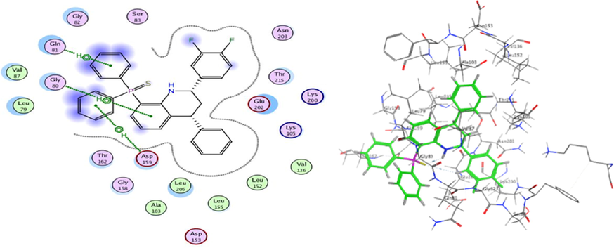
3D docking and 2D of compound C26 and 6G77 protein cancer of lung cancer protein.
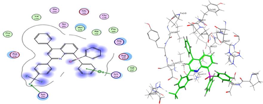
3D docking and 2D of compound C11 and 2NS2 protein cancer of ovarian cancer protein.
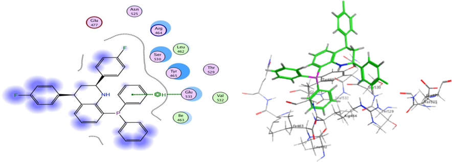
3D docking and 2D of compound C19 and 5 K47 protein cancer of kidney cancer protein.
3.7 Molecular dynamics simulation
In order to test the stability of the three most active ligands (molecules C11, C19 and C26), dynamic molecular modeling was performed for 10 ns. Fig. 13 displays the conformational changes of the three ligands.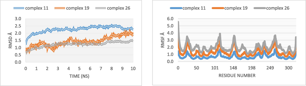
RMSD and RMSF of molecular dynamics results.
Using three complexes 11, 19, and 26 designated respectively 2NS2-C11, 5 K47-C19, and 6G77-C26 built for the target protein to assure the projected binding stability of the complex system, a 10 ns molecular dynamic simulation of the interactions between three docked molecules was run. Fig. 13 shows that during the MD simulations, the RMSD of the complex 11 ranged between 2.2 and 2.5 Å, with the average RMSD from 0 to 3 ns being found to be 1 Å. After the complex's curve slightly increased to a value of about 2.45 Å, the complex's system became equilibrated for the remaining time. According to the RMSD analysis, the target protein for complexes 19 and 26 ranged between 1 and 1.9 Å over the MD simulations, with an average RMSD of 1.5 Å.
As a result, the Rg figure demonstrates that following molecule binding, the target protein's folding compactness has not significantly changed Fig. 14. The outcomes after reviewing the MD simulation diagram supported the earlier molecular docking outcomes. Since there was little fluctuation in the properties of the three selected ligands, they were able to build dynamically stable connections with their proteins for the simulation time of 10 ns.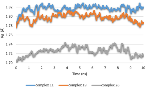
The radius of gyration of the molecular dynamics results.
4 Conclusion
In the present work, the proliferative activity of Topoisomerase I Inhibitors in a series of 28 phosphorus substituted quinoline derivatives was investigated and electronic descriptors in addition to Lipinski parameters were used to relate them to biological activity. The stability and predictive power was confirmed by internal and external validation. It is worth mentioning that the docking study was made to investigate the interaction of the most active compounds with three proteins: 6G77, 2NS2 and 5 K47. The findings show that hydrogen and pi-cation interactions with the ester function and the triofluromethyl group (-CF3) have a great effect on the activity values studied, which confirms the experimental results. Based on the computational analyses, compounds C11, C19 and C26 were found to have maximum binding affinity to the target proteins of ovarian, kidney and lung cancers, respectively. The three chosen ligands created dynamically stable connections with respective proteins during the 10 ns simulation time. Based on the above facts, the three compounds may be offered to be key structures for the design and synthesis of newer and more powerful anti-cancer drugs.
References
- Polymer complexes. LXXV. Characterization of quinoline polymer complexes as potential bio-active and anti-corrosion agents. Mater. Sci. Eng. C. 2019;103
- [Google Scholar]
- DFT-based QSAR study of substituted pyridine-pyrazole derivatives as corrosion inhibitors in molar hydrochloric acid. Int. J. Electrochem. Sci.. 2014;9(9):4732-4746.
- [Google Scholar]
- Chloroquine analogs as antimalarial candidates with potent in vitro and in vivo activity. Int. J. Parasitol.: Drugs Drug Res.. 2018;8(3):459-464.
- [Google Scholar]
- Novel topoisomerase I inhibitors. Syntheses and biological evaluation of phosphorus substituted quinoline derivates with antiproliferative activity. Eur. J. Med. Chem.. 2018;149:225-237.
- [Google Scholar]
- Global cancer facts & figures (4th edition). Atlanta, GA: American Cancer Society; 2018.
- Density-functional exchange-energy approximation with correct asymptotic behavior. Phys. Rev.. 1988;38:3098-3100.
- [Google Scholar]
- Density functional thermochemistry. I, the effect of the exchange only gradient correction. J. Chem. Phys.. 1992;96:2155-2160.
- [Google Scholar]
- Design, synthesis, and evaluation of new 2-(quinoline-4-yloxy) acetamide-based antituberculosis agents. Eur. J. Med. Chem.. 2020;192:112179
- [Google Scholar]
- Synthesis and Analgesic Activity of [b]-Annelated 4-Quinolones. Pharm. Chem. J.. 2019;53(7):616-619.
- [Google Scholar]
- Global cancer statistics 2018: GLOBOCAN estimates of incidence and mortality worldwide for 36 cancers in 185 countries. CA Cancer J. Clin.. 2018;68:394-424.
- [Google Scholar]
- QSAR study of unsymmetrical aromatic disulfides as potent avian SARS-CoV main protease inhibitors using quantum chemical descriptors and statistical methods. Chemom. Intell. Lab. Syst.. 2021;210:104266
- [Google Scholar]
- Chloroquine and hydroxychloroquine as available weapons to fight COVID-19. Int. J. Antimicrob. Agents. 2020;105932(10.1016)
- [Google Scholar]
- Khan, Descriptors and their selection methods in QSAR analysis: paradigm for drug design. Drug Discov. Today. Aug. 2016;21(8):1291-1302.
- [Google Scholar]
- Principal component analysis: a method for determining the essential dynamics of proteins. In: Protein Dynamics. Springer; 2014. p. :193-226.
- [Google Scholar]
- Quantum chemical and QSPR studies of bis-benzimidazole derivatives as corrosion inhibitors by using electronic and lipophilic descriptors. Desalin. Water Treat.. 2018;111:208-225.
- [Google Scholar]
- Computational study and qspr approach on the relationship between corrosion inhibition efficiency and molecular electronic properties of some benzodiazepine derivatives on c-steel surface. Analytical and Bioanalytical Electrochemistry. 2019;11(3):373-395.
- [Google Scholar]
- QSAR, ADMET In Silico Pharmacokinetics, Molecular Docking and Molecular Dynamics Studies of Novel Bicyclo (Aryl Methyl) Benzamides as Potent GlyT1 Inhibitors for the Treatment of Schizophrenia. Pharmaceuticals. 2022;15:670.
- [Google Scholar]
- Polymer complexes. LXXVI. Synthesis, characterization, CT-DNA binding, molecular docking and thermal studies of sulfoxine polymer complexes. Appl. Organometallic Chem.. 2019;33(5)
- [Google Scholar]
- 3D-QSAR Studies, Molecular Docking, Molecular Dynamic Simulation, and ADMET Proprieties of Novel Pteridinone Derivatives as PLK1 Inhibitors for the Treatment of Prostate Cancer. Life. 2023;13:127.
- [Google Scholar]
- Targeting of TMPRSS4 sensitizes lung cancer cells to chemotherapy by impairing the proliferation machinery. Cancer Lett.. 2019;453:21-33.
- [Google Scholar]
- Targeted enhancement of flotillin-dependent endocytosis augments cellular uptake and impact of cytotoxic drugs. Sci. Rep.. 2019;9(1):1-15.
- [Google Scholar]
- Anti-inflammatory quinoline alkaloids from the root bark of Dictamnus dasycarpus. Phytochemistry. 2020;172:112260
- [Google Scholar]
- Comparative molecular field analysis and hologram quantitative structure activity relationship studies of pyrimidine series as potent phosphodiesterase 10A inhibitors. J. Chin. Chem. Soc. 2018
- [Google Scholar]
- Molecular docking and receptor-based QASR studies on pyrimidine derivatives as potential phosphodiesterase 10A inhibitors. Struct. Chem. 2019
- [Google Scholar]
- Computational Modeling of Novel Phosphoinositol-3-Kinase Inhibitors Using Molecular Docking, Molecular Dynamics, and 3D-QSAR. Bull. Kor. Chem. Soc.. 2021;42:1093-1111.
- [Google Scholar]
- Structure activity and prediction of biological activities of compound (2-methyl-6-phenylethynylpyridine) derivatives relationships rely on electronic and topological descriptors. J. Comput. Methods Mol. Des.. 2014;4:61-71.
- [Google Scholar]
- https://www.rcsb.org/pdb/welcome.do.
- Cell Division, Cytotoxicity, and the Assays Used in the Detection of Cytotoxicity. Cytotoxicity-Definition: Identification, and Cytotoxic Compounds, IntechOpen; 2019.
- Anticancer, antimicrobial activities of quinoline based hydrazone analogues: synthesis, characterization and molecular docking. Bioorg. Chem.. 2020;94:103406
- [Google Scholar]
- QSAR modeling and molecular docking studies of 2-oxo-1, 2-dihydroquinoline-4-carboxylic acid derivatives as p-glycoprotein inhibitors for combating cancer multidrug resistance. Heliyon. 2023;9(1):e13020
- [Google Scholar]
- Development of the Colle-Salvetti conelation energy formula into a functional of the electron density. Phys. Rev. B. 1988;37:785-789.
- [Google Scholar]
- Synthesis and colon anticancer activity of some novel thiazole/-2-quinolone derivatives. J. Mol. Struct.. 2020;1207:127798
- [Google Scholar]
- Probing the binding mechanism of capecitabine to human serum albumin using spectrometric methods, molecular modeling, and chemometrics approach. Bioorg. Chem.. 2019;90:103037
- [Google Scholar]
- Recent studies of antioxidant quinoline derivatives. Mini Rev. Med. Chem.. 2013;13(3):365-372.
- [Google Scholar]
- Antimicrobial and antiproliferative activity studies of some new quinoline-3-carbaldehyde hydrazone derivatives. Bioorganic Chem.. 2020;104014
- [Google Scholar]
- Predicting soil phosphorus and studying the effect of texture on the prediction accuracy using machine learning combined with near-infrared spectroscopy. Spectrochimica Acta - Part A: Molecular and Biomolecular Spectroscopy. 2020;242:118736
- [Google Scholar]
- Isobaric and Isothermal Molecular Dynamics Simulations Utilizing Density Functional Theory: An Assessment of the Structure and Density ofWater at Near-Ambient Conditions. J. Phys. Chem. B. 2009;113:11959-11964.
- [Google Scholar]
- Mechanisms of action of hydroxychloroquine and chloroquine: implications for rheumatology. Nature 2020:1-12.
- [Google Scholar]
- Antiinflammatory and antiarthritic properties of a substituted quinoline carboxylic acid: CL 306,293. J. Rheumatol.. 1991;18(6):855-860.
- [Google Scholar]
- STATITCF Software, Technical Institute of Cereals and Fodder, Paris, France, 1987.
- Quinoline derivatives: potential antiparasitic and antiviral agents. Acta Crystallogr. C. 2007;63(11):o643-o645.
- [Google Scholar]
- An Effective Solvation Term Based on Atomic Occupancies for Use in Protein Simulations. Mol. Simul.. 2006;10:97-120.
- [Google Scholar]
- Cancer cachexia—pathophysiology and management. J. Gastroenterol.. 2013;48(5):574-594.
- [Google Scholar]
- Synthesis of quinoline derivatives as diabetic II inhibitors and molecular docking studies. Bioorg. Med. Chem.. 2019;27(18):4081-4088.
- [Google Scholar]
- Chemometrics tools in QSAR/QSPR studies: a historical perspective. Chemom. Intell. Lab. Syst.. Dec. 2015;149:177-204.
- [Google Scholar]
Appendix A
Annex 1:
Abbreviation of molecular descriptors
description
E LUMO
Highest occupied molecular orbital energy
E HOMO
Lowest unoccupied molecular orbital energy
lip_acc
Lipinski acceptor count
logP (o/w)
Log octanol/water partition coefficient
E l-h
Energy gap
KierFlex
Molecular flexibility
μ
Dipole moment
S
Softness
χ
Electronegativity
I
Ionization potential
A
Electron affinity
η
Hardness
dens
Density
Abbreviation
description
S
The finale score of GBVI/WSA binding free energy
Rmsd_refine
The mean square deviation after refinement
E_place
Score of the placement phase
E_conf
Energy conformer
E_refine
Score refinement
E_scor1
Score the first step of notation
Compounds
pIC50
E LUMO
E HOMO
E l-h
KierFlex
logP (o/w)
μ
S
χ
I
A
η
dens
dipole
lip_acc
1
−0.24
−1.69
−5.93
−4.24
4.77
7.68
−3.81
0.24
3.81
5.93
1.69
2.12
0.98
1.14
2.00
2
−0.43
−1.77
−5.94
−4.18
4.93
7.83
−3.86
0.24
3.86
5.94
1.77
2.09
1.02
0.97
2.00
3
0.30
−2.65
−3.63
−0.98
5.48
8.61
−3.14
1.02
3.14
3.63
2.65
0.49
1.07
0.98
2.00
4
−0.58
−1.09
−3.33
−2.24
4.74
6.41
−2.21
0.45
2.21
3.33
1.09
1.12
1.00
1.79
3.00
5
0.68
−1.71
−5.87
−4.17
5.38
7.63
−3.79
0.24
3.79
5.87
1.71
2.08
0.99
1.39
3.00
6
−0.55
−2.05
−5.57
−3.51
4.94
8.90
−3.81
0.28
3.81
5.57
2.05
1.76
0.99
1.15
2.00
7
0.60
−1.82
−5.99
−4.16
5.10
7.98
−3.90
0.24
3.90
5.99
1.82
2.08
1.04
1.23
2.00
8
−0.08
−1.87
−5.57
−3.70
4.99
7.98
−3.72
0.27
3.72
5.57
1.87
1.85
0.98
1.17
2.00
9
−0.08
−1.80
−6.03
−4.23
4.28
8.25
−3.92
0.24
3.92
6.03
1.80
2.11
0.99
1.25
2.00
10
−0.35
−1.85
−6.02
−4.17
4.44
8.40
−3.94
0.24
3.94
6.02
1.85
2.08
1.02
1.24
2.00
11
−0.01
−2.03
−6.31
−4.28
4.98
9.18
−4.17
0.23
4.17
6.31
2.03
2.14
1.08
1.30
2.00
12
−0.47
−1.88
−6.15
−4.27
4.25
7.17
−4.01
0.23
4.01
6.15
1.88
2.14
1.01
0.98
3.00
13
−0.49
−1.67
−5.74
−4.06
4.86
8.20
−3.70
0.25
3.70
5.74
1.67
2.03
1.00
1.30
3.00
14
−0.80
−1.83
−5.61
−3.78
4.49
9.47
−3.72
0.26
3.72
5.61
1.83
1.89
1.00
1.27
2.00
15
−0.58
−1.91
−6.07
−4.16
4.60
8.55
−3.99
0.24
3.99
6.07
1.91
2.08
1.05
0.87
2.00
16
−0.88
−1.76
−5.99
−4.23
4.49
8.55
−3.88
0.24
3.88
5.99
1.76
2.12
0.99
1.28
2.00
17
0.22
−0.48
−5.32
−4.83
4.72
8.05
−2.90
0.21
2.90
5.32
0.48
2.42
0.96
0.16
1.00
18
−1.21
−0.70
−5.38
−4.68
5.43
8.99
−3.04
0.21
3.04
5.38
0.70
2.34
1.04
0.47
1.00
19
1.10
−0.59
−5.18
−4.59
5.05
8.36
−2.89
0.22
2.89
5.18
0.59
2.30
1.02
0.33
1.00
20
0.96
−0.48
−5.03
−4.55
4.94
8.35
−2.75
0.22
2.75
5.03
0.48
2.28
0.95
0.20
1.00
21
0.60
−0.53
−5.10
−4.57
5.10
8.50
−2.81
0.22
2.81
5.10
0.53
2.29
0.98
0.43
1.00
22
−0.39
−0.44
−4.97
−4.53
5.56
8.31
−2.71
0.22
2.71
4.97
0.44
2.26
0.96
0.43
2.00
23
0.80
−1.73
−4.18
−2.45
5.24
8.88
−2.95
0.41
2.95
4.18
1.73
1.22
0.98
1.44
1.00
24
0.66
−2.06
−4.42
−2.36
5.96
9.81
−3.24
0.42
3.24
4.42
2.06
1.18
1.06
1.17
1.00
25
0.57
−1.76
−4.23
−2.47
5.41
9.03
−2.99
0.41
2.99
4.23
1.76
1.23
1.01
1.26
1.00
26
1.10
−1.88
−4.34
−2.46
5.57
9.22
−3.11
0.41
3.11
4.34
1.88
1.23
1.05
1.25
1.00
27
0.57
−1.85
−4.18
−2.32
5.38
10.14
−3.01
0.43
3.01
4.18
1.85
1.16
0.99
1.42
1.00
28
1.52
−1.81
−4.27
−2.46
5.57
9.18
−3.04
0.41
3.04
4.27
1.81
1.23
1.04
1.08
1.00
Appendix B
Supplementary data
Supplementary data to this article can be found online at https://doi.org/10.1016/j.arabjc.2023.104783.
Appendix B
Supplementary data
The following are the Supplementary data to this article:Supplementary data 1
Supplementary data 1


